SimQuick process simulation with excel sach scan
Bạn đang xem bản rút gọn của tài liệu. Xem và tải ngay bản đầy đủ của tài liệu tại đây (7.27 MB, 125 trang )
SimQuick
Process Simulation with Excel
Third Edition
David Hartvigsen
Mendoza College of Business
UniversitY ofNotre Dame
(Updated on 6/15/2016)
Copyright © 2016 by David Hartvigsen
Updated on 6/15/2016
All rights reserved. No part of this publication may be reproduced, distributed, or transmitted
in any form or by any means, including photocopying, recording, or other electronic or
mechanical methods, without
prior written permission of the author, except in the case
brief quotations embodied in critical reviews and certain other noncommercial uses permitted
by copyright law. For permission requests, write to the author at
David Hartvigsen
Mendoza College of Business
University of Notre Dame
Notre Dame, IN 46556
Email:
To order, go to Amazon.com
Printed by CreateSpace, Charleston, SC
This book was previously published by: Pearson Education, Inc.
2
To Nancy
3
Table of Contents
Preface ........................................................................................................ 7
Motivation ....... .. ............. .. .... ... .. ... ... ..... .. .. .. .. .... .. .. .......... .... .. ... .. ... ... .. 7
How to use the booklet ..................................................................... 8
Chapter 1: Introduction ...................................................................... 11
Sec.
Sec.
Sec.
Sec.
1:
2:
3:
4:
What is process simulation? .................................................
What does SimQuick do? .....................................................
How does SirnQuick incorporate uncertainty? ... .. .. ... .. .. ... ....
System requirements and "installation" ................................
12
13
14
16
Chapter 2: Waiting Lines ................................................................... 18
Sec. 1: Solving a problem with SimQuick ........................................ 19
Example 1: A Bank ....... .. ... ... .. .. .. .. .. ...... .. .. ... ... .. ... .. .. ... ... .. ..... 19
Modeling the process (with a process flow map) .....
Entering the model into SimQuick ...........................
Interpreting SimQuick results ...................................
Improving the process, Variation 1 ...........................
Improving the~process, Variation 2 ...........................
20
20
26
29
31
Sec. 2: Additional waiting line processes ......................................... 33
Example 2: A grocery store checkout ................................... 33
Example 3: A call center ...................................................... 34
Example 4: A fast-food restaurant drive-thru ....................... 35
Sec. 3: Decision Points ...................................................................... 35
Example 5: An airport security system ................................. 36
Example 6: A department of motor vehicles ........................ 39
Example 7: A hospital emergency room ............................... 41
Sec. 4: Advanced SimQuick features .............................................. 42
Example 8: Buffer Tracking .................................................
Example 9: "Unavailable" elements .....................................
Example 10: Changing Distributions ...................................
Example 11: Discrete Distributions ......................................
4
43
44
45
48
Example 12: Resources and Priorities .................................. 50
Chapter 3: Inventory in Supply Chains ........................................ 54
Sec. 1: A periodic review inventory policy ....................................... 56
Example 13: Grocery store inventory .. .. .. .. .. ... ...... .. ... ...... .. .. . 56
Sec. 2: Reorder point inventory policies ........................................... 59
Example 14: An electronics superstore ................................ 59
Example 15: A warehouse ...... .. .. .. ..... .. ........ ..... .. ... ......... .. ... . 63
Example 16: Two stores and a warehouse ............................ 64
Sec. 3: More complex inventory policies .... ....... .. .. .. .. ... .. ... .... .... .. ... . 66
Example 17: An appliance store .... .. .. .. ... .. .... ... .. ... .. .. .. .. .... .. .. 67
Example 18: A department store .......................................... 72
Chapter 4: Manufacturing ................................................................. 78
Sec. 1: Linear flow processes ... ... .... .. .... .. .......... .. .. .. .. .... ..... ... ........ .. . 79
Example 19: A generic linear flow process .......................... 80
Example 20: A manufacturing cell ....................................... 82
Sec. 2: Assembly/disassembly proc~sses .......................................... 84
Example 21: Box manufacturing ... .. ... .. ........... .. ..... ............. . 84
Sec. 3: Batch and job shop processes ............................................... 87
Example 22: Pharmaceutical manufacturing ........................ 88
Example 23: A single machine job shop .............................. 91
Sec. 4: Quality and reliability in processes ....................................... 94
Example 24: A quality control station .................................. 94
Example 25: A machine with breakdowns .... .. .. .. ....... .... .. .. .. 97
Chapter 5: Project Management ..................................................... 98
Example 26: A software development project ........................... 99
Example 27: A house addition project ....................................... 103
5
Appendix 1: The Steps in a Simulation Project ......................... 105
Appendix 2: Enhancing SimQuick with Excel Features ......... 106
Appendix 3: Scenarios ......................................................................... 108
Appendix 4: Custom Schedules ........................................................ 113
Appendix 5.: SimQuick Reference Manual .................................. 116
6
Preface
Motivation
The simulation of processes (waiting lines, factories, supply chains, and so on) is one of the
conceptually simplest and most often applied techniques in Operations Management and
Management Science, yet it has not been widely taught to business students. A key reason for
this is that performing process simulation requires the use of software, and the software that is
available tends to be complex and expensive. Even the more graphics-based packages, although
often beautifully designed, frequently have an enormous number of features that place an
unnecessary burden on students (and instructors) in classes that are not devoted to simulation.
SimQuick is an Excel-based software package for process simulation that is easy to learn, easy to
use, and freely distributed. (Its key features can be learned in an hour or two of class time or
independent reading.) It is an ordinary Excel file with some hidden macros and should run
immediately on any modem personal or networked computer that runs Excel, either a PC or an
Apple computer; it is not an "add-in" and requires no "installation." Hence, users of Excel will
already be familiar with much of the interface, and the results are already in the spreadsheet,
ready for analysis.
SimQuick is aimed primarily at business students and managers who want to quickly learn the
basics of process simulation and be able to quickly analyze and improve real-world processes.
SimQuick is flexible in its modeling capability; that is, it is not a "hardwired" set of examples; it
requires true modeling. The user can combine the basic building blocks of SimQuick in a huge
variety of ways. Hence, SimQuick can serve well as an introduction to both the notion of
building quantitative models as well as the important field of simulation. Since the first version
of SimQuick was released in 2001, it has been used in industry as well as in the classroom; its
original design and subsequent updates have been informed by comments from users in both
domains.
This (inexpensive) booklet accompanies SimQuick. It presents the basics of process simulation
by having the reader construct, run, and analyze simulations of realistic processes using
SimQuick. An emphasis has been placed on explaining precisely how the various building
blocks of SimQuick work. Chapter 1 contains a brief introduction to process simulation and the
concepts underlying SimQuick. The next four chapters contain a variety of examples of process
simulation. These examples are organized as follows: waiting lines (Chapter 2), inventory in
supply chains (Chapter 3), manufacturing (Chapter 4), and project management (Chapter 5).
Each example is followed by an exercise. All of the examples and exercises have been designed
with business students and managers in mind.
In addition to presenting the basics of process simulation, this booklet introduces a number of key
concepts from the analysis of processes: service level, cycle (or waiting) time, throughput,
bottleneck, batch size, setup, priority rule, and so on. The booklet also introduces some key
trade-oifs from the analysis of processes: number of servers vs. service level, inventory level vs.
7
service level, working time variability vs. throughput, batch size vs. service level, and so on.
These notions are presented through computer models that the reader constructs and experiments
with using SimQuick.
How to use the booklet
The booklet is self-contained; that is, all technical terms involving processes or operations are
defined. The reader is assumed to have a rudimentary understanding of how to use Excel on the
level of knowing how to save files and how to enter information into cells. Also, a basic
understanding of statistical distributions, such as the normal distribution, would be helpful. The
chapters are organized around typical topics in Operations Management and Spreadsheet
Modeling courses so that this booklet can easily be used in these types of courses.
The reader should first read Chapter 1 (which contains a conceptual explanation of process
simulation and SimQuick) and Section 1 of Chapter 2 (which contains a step-by-step explanation
of how to use SimQuick by completely working through a simple example). After this, the
reader has a lot of freedom (with some Examples recommended as prerequisites in a few spots).
Chapters 2 through 5 consist of examples of processes that can be modeled using SimQuick.
When needed, an example discusses how to build the SimQuick model. Each example is
followed by an exercise.
A quick treatment of process simulation could consist of working through Example/Exercise 1
for waiting lines and Example/Exercise 19 for manufacturing. With just this material, many realworld processes can be easily modeled and studied. Adding Example/Exercise 5 with Decision
Points would allow the modeling of 1pany more types of processes. A reading of Examples 8, 9,
and 10 would introduce the notion of Changing Distributions and further increase the variety of
real-world processes that can be modeled. Adding Examples/Exercises 13 and 14 would provide
a quick introduction to the modeling of inventory in supply chains and adding Example/Exercise
26 would serve as an introduction to the incorporation of uncertainty into project management
models.
The booklet contains five appendices. Appendix 1 contains a list of the basic steps in conducting
a simulation project. Appendix 2 contains tips on how to enhance SimQuick by using some of
the features built into Excel. A tool with wide applicability, called Scenarios, is discussed in
Appendix 3, where references are made to several Examples/Exercises from the text. Appendix
4 describes how to use a feature of SimQuick called Custom Schedules. Appendix 5 contains a
succinct description of all the features of SimQuick and can be used for reference. Hence, the
features of SimQuick are presented in two ways: through examples and in a reference manual.
Solutions to exercises: Instructors can obtain solutions to every exercise. To obtain solutions, an
instructor should send a request to the author () with a copy of their course
syllabus and a link to their webpage at their educational institution.
8
Web site: Refer to SimQuick.net for additional information on SimQuick, this booklet, and
technical support.
Over the past 15 years, I have used SimQuick in the classroom with executive MBAs, full-time
MBAs, and undergraduate business students. After a one-hour introduction in class (basically,
covering Section 1 of Chapter 2), the students successfully solve a variety of modeling problems
with little help. This introduction has also served as a launching pad for term projects, whereby
students identify and analyze real-world processes of their choice.
New to the 3rd edition:
The SimQuick software and booklet have been updated in several ways in this
are the key updates:
•
•
•
•
•
•
•
•
3rd
edition. Here
Due to improvements in the SimQuick software and the steady advance of computer
hardware, SimQuick runs considerably more quickly than when the 2nd edition appeared.
This allows more simulations to be performed in a reasonable amount of time, which
leads to more accurate results. Hence, more simulations are allowed and recommended in
the examples/exercises.
A new feature called Scenarios has been added. This feature allows you to easily test, at
one time, multiple variations on a given model and then compare the results in one
worksheet. This feature is described in the new Appendix 3 with examples from the text.
Another new feature called Changing Distributions allows a statistical distribution to
change during the course of a simulation. With this, you can model, for example,
customer arrival rates that increase and decrease during the span of a simulated day. This
feature is illustrated in Example/Ex~rcise 10, which is new to this edition.
Models can now allow Work Stations, Entrances, and Exits to be "available" or
"unavailable" during a simulation. With this feature you can more easily experiment with
the number of workers or machines that are available during a simulation. This feature
can also be combined with Changing Distributions to allow a worker or machine, for
example, to be available during only some time periods during a simulation. This feature
is illustrated in the newly added Examples/Exercises 9 and 10.
With a new feature called Buffer Tracking you can display how inventory levels (of
people or products) vary during a simulation. This allows you, for example, to pinpoint
where and when bottlenecks occur, which allows, for example, more accurate
adjustments of staffing levels or numbers of machines. This feature is introduced in the
newly added Example/Exercise 8 and elaborated in Example/Exercise 10.
Data entry has been simplified and streamlined with the introduction of pull-down lists
within most cells of the data entry tables.
The discussion of how to perform statistical analyses of SimQuick output (in Appendix 2)
has been updated and streamlined by making use of Excel's built in statistical functions.
You now have the option to specify a "seed" before starting a run of simulations. By
doing this the same sequence of random numbers can be generated each time a group of
simulations is run. (However, please note that the sequences are chosen differently on
PCs and Apple machines.)
9
Acknowledgments
The design of SimQuick was inspired by the breakthrough simulation product X CELL, so I want
to begin by acknowledging its authors: Richard Conway, William L. Maxwell, John 0. McClain,
and Steven L. Worona. Next, I want to thank the editor Tom Tucker at Prentice Hall, who
worked with me on the first two editions. He was indispensable in helping me to define this
project and bring it to fruition. I want to thank the following reviewers for their careful reading
and excellent suggestions on a draft of the first edition: Sue Abdinnour-Helm, Arundhati Kumar,
Larry Meile, Kelly B. Nichols, Jeffrey L. Rummel, and Billy M. Thornton. I want to thank
Kristin Arin Steffeck for her copy editing on the first edition. I'd also like to thank the reviewers
of the second edition for their thoughtful suggestions based on their classroom use of SimQuick:
C.H. Aikens, Stephen N. Chapman, Christos Koulamas, Michael Schwartz, and Billy M.
Thornton. I want to thank my colleagues Lee Krajewski and Hojung Shin for a number of
helpful discussions of this project in its early stages and I want to thank my colleagues Yanjun
Li, Jerry Wei, and Hong Guo for their suggestions for this third edition. I also want to thank
Robert Maurer, Fazel Hayati, and Jeffery Brach for some very helpful discussions of the third
edition. Finally, I want to thank my many students (executive MBAs, full-time MBAs, and
undergraduate business students) of the past 15 years who have made many helpful suggestions
during the development of this software and booklet. In particular, I'd like to single out Douglas
Wait, Ben Gaw, Patrick Dahman, Xuejun Zhang, and Katy Delany for their insights.
10
Chapter 1: Introduction
Learning objectives:
•
•
•
•
To understand the idea of process simulation.
To understand the general structure of SimQuick models.
To understand the role of uncertainty in process simulation.
To get SimQuick running on your computer.
11
Overview
This chapter contains a brief defmition of process simulation, an overview ofhow SimQuick
works, and instructions for how to run SimQuick on a computer. Most of the details of how to
use SimQuick are covered in Chapter 2, Section 1.
Section 1: What is process simulation?
Process simulation is a widely used technique for improving the efficiency of processes.
Following are some examples of processes and some related efficiency problems that can be
addressed with process simulation (and SimQuick):
Examples of processes:
•
•
•
•
•
•
People moving through a bank or post office.
Telephone calls moving through a call center.
Parts moving along an assembly line or through a batch process or job shop.
Inventory moving through a retail store or warehouse.
Products moving by trucks, trains, planes, or ships through a supply chain.
A software development project.
Examples of efficiency problems:
•
•
•
•
•
•
•
•
•
How many tellers are needed to keep waiting times at a bank reasonably short?
What effect will a new answering system have on how long customers wait at a call center?
What effect will a new just-in-t'ime (JIT) inventory system have on the number of units
produced per day on an assembly line?
What is the best batch size to use in a factory?
What is the best delivery policy for goods at a warehouse?
How much inventory should be kept on the shelves in a grocery store?
How many machines should each worker operate in a manufacturing cell?
How should inventory be distributed along a supply chain?
What is the expected duration of a software development project?
With process simulation, you begin by building a computer model of a real-world process. Your
initial goal is to have the computer model behave in a way similar to the real process, except
much more quickly. You then try out various ideas for efficiency improvements on the computer
model and use the best ideas on the real process. Thus, a lot of time and money can be saved.
Simulation is particularly useful when there is uncertainty in a process: for example, the arrival
times of customers, the demand for a product, the supply of parts, the time it takes to perform the
work, the quality of the work. With uncertainty, it is often difficult to predict the effects of
making changes to a process, especially if there are two or more sources of uncertainty that
interact.
12
Section 2: What does SimQuick do?
SimQuick allows you to perform process simulation within the Excel spreadsheet environment.
There are three basic steps involved in using SimQuick. (For a more detailed list of steps, see
Appendix 1.)
1.
Conceptually build a model of the process using the building blocks of SimQuick
(introduced below).
2.
Enter this conceptual model into SimQuick. (This is done by filling in tables in a special
Excel spreadsheet.)
3.
Test process improvement ideas on this computer model.
The building blocks in SimQuick are objects, elements, and statistical distributions. Objects
typically represent things that move in a process: people, parts in a factory, paperwork, phone
calls, e-mail messages, and so on. Elements typically represent things that are stationary in a
process. There are five types of elements:
Entrances: This is where objects enter a process. Entrances can represent a loading dock at a
warehouse, a door at a store, and so on. You must specify when objects arrive at an Entrance and
in what numbers (using a statistical distribution or an explicit "custom" schedule).
Buffers: This is where objects can be stored. Buffers can represent a location in a warehouse or
factory where inventory can be stored, a place where people can stand in line at a post office, a
memory location in a computer for e-mail messages, and so on. You must specify how many
objects a Buffer can hold.
Work Stations: This is where work is performed on objects. Work Stations can represent
machines in a factory, cashiers in a store, operators at a call center, computers in a network, and
so on. You must specify how long a Work Station works on an object (using a statistical
distribution).
Decision Points: This is where an object goes in one of two or more (up to 10) directions.
Decision Points can represent the outcome of a quality control station, different routings in the
processing of a mortgage application, and so on. You must specify a rule for deciding in which
direction an object goes (using a statistical distribution).
Exits: This is where objects leave a process. Exits can represent a loading dock at a warehouse, a
customer buying a product at a store, and so on. You must specify when objects depart from an
Exit and in what numbers (using a statistical distribution or an explicit "custom" schedule).
13
The third building block, statistical distributions, is discussed in the next section.
A SimQuick model describes how the objects move between the elements. You have a great deal
of freedom in constructing models using the building blocks of SimQuick; hence, you can model
a variety of real processes. Because the building blocks in SimQuick are intentionally simple, it
is best suited to modeling processes of low to intermediate complexity.
When a SimQuick simulation begins, a "simulation clock" starts in the computer and runs for the
designated duration of the simulation. While this clock is running, a series of simulation events
takes place sequentially. There are three types of simulation events in SimQuick: the arrival of
objects at an Entrance, the departure of objects from an Exit, and the finish of work on an object
at a Work Station. Whenever an event occurs, SimQuick moves objects from element to element
as much as possible. SimQuick keeps track of various statistics during the simulation (e.g., the
mean inventory at each Buffer) so you can analyze what happened when the simulation is over.
Section 3: How does SimQuick incorporate uncertainty?
As in a real process, the timing of events in SimQuick can be uncertain or random. Here is an
example: Suppose you are entering a model into SimQuick that contains a Work Station. You
must specifY how much time this Work Station works on an object. What do you do if this time
varies in a random fashion at the real work station? A typical approach is to observe the real
work station and record a list of real working times. Following are four common possibilities
and the ways in which SimQuick models them.
Case 1: The list of real working times has a "bell-shaped" histogram:
Histogram
40
35
;:... 30
g
25
~ 20
[ 15
LL 10
5
0
cV
'\Ql "' ~
~·
~·
~·
Real working times
Note: The height of each bar represents the number of observed working times that fall into the
interval indicated at the base of the bar on the horizontal axis.
Then, a list of numbers taken randomly from a normal distribution, with the same mean and
standard deviation as your list, is likely to have a similar-looking histogram. So, for example, if
14
your list of numbers has a mean of 3 minutes and a standard deviation of 1 minute, then you
would enter Nor(3,1) into SimQuick. Thus, you are instructing SimQuick to randomly pick each
working time for this Work Station from the normal distribution with mean of 3 and standard
deviation of 1.
Case 2: The list of real working times has a histogram that is "skewed to the right" as follows:
Histogram
100
~
tT
80
60
40
LL
20
;
::1
!!!
0
Real working times
Then, a list of numbers taken randomly from an exponential distribution, with the same mean as
your list, is likely to have a similar-looking histogram. So, for example, if your list of numbers
has a mean of 3 minutes, then you would enter Exp(3) into SimQuick. Thus, you are instructing
SimQuick to randomly pick each working time for this Work Station from the exponential
distribution with mean of 3.
Case 3: The list of real working times has a histogram whose bar heights are all roughly the
same:
Histogram
~ 40
1:: 30
~ 20
g
U:
10
0
Real working times
Then, a list of numbers taken randomly from a uniform distribution, with the same minimum and
maximum values as your list, is likely to have a similar-looking histogram. So, for example, if
your list of numbers has minimum and maximum values of 1 and 6, then you would enter
Uni(1,6) into SimQuick. Thus, you are instructing SimQuick to randomly pick each working
15
time for this Work Station from the uniform distribution with minimum and maximum values of
1 and 6.
Case 4: The list of real working times can be described by a histogram with at most ten bars:
Histogram
~ 30
;
tT
20
10
I.L
0
::::1
~
0
1
2
3
4
5
6
7
8
Real working times
A discrete distribution in SimQuick has up to ten output numbers, each chosen with a specified
probability. To model a histogram, we choose one number from each interval as an output
number (as shown above) and we set its probability to be proportional to the height of its bar.
Then, a list of numbers taken randomly from this output list, according to the associated
probabilities, is likely to have a similar-looking histogram. In SimQuick this is modeled with the
Dis function.
The details of how to use the "Nor," "Exp," "Uni," and "Dis" functions are provided in Chapters
2 through 5 and Appendix 5. To input fixed schedules, see Appendix 4.
Section 4: System requirements and "installation"
System requirements: To run SimQuick, you must be able to run Microsoft Excel on your
computer. (Excel can run from your hard drive or from a network.) In particular, you need to
have Excel2003 or later on a PC, or Excel2011 or later on an Apple computer.
"Installing" and running SimQuick: Go to the website SimQuick.net and download a copy of
SimQuick-v3. It is a standard Excel spreadsheet file (with some special worksheets and macros).
To use SimQuick, simply open this file or launch the application Excel and, within Excel, open
the file. You are now ready to go!
Note on security: When opening SimQuick-v3, you may see "Security Warning" with a button
labelled "Enable Content" or "Enable Macros." You may also see a button labelled "Enable
Editing." In all such cases, just click the button. If Excel does not allow you to enable the
SimQuick macros, go to SimQuick.net for some pointers.
It is probably most convenient to put a copy of SimQuick-v3 on your computer or network space
and open this copy when you want to use SimQuick.
16
Saving a SimQuick model: After opening SimQuick-v3, you may save your work at any time just
as you do with any Excel spreadsheet: Simply click on "Save As" under the "File" menu. You'll
probably want to rename SimQuick-v3 and specify a location on your computer or network
space.
If a problem arises with your copy ofSimQuick-v3 (e.g., the formatting gets changed or a
worksheet gets deleted), just replace it with a fresh copy from the website or your storage space.
17
Chapter 2: Waiting Lines
Learning objectives:
•
•
•
•
•
•
•
To understand the basics of using SimQuick.
To model, simulate, and analyze a variety of waiting line processes.
To understand the following performance measures: service level, mean cycle (or waiting)
time, and mean inventory (or number of customers in line).
To analyze the trade-off between number of servers and service level.
To understand the SimQuick elements: Entrances, Work Stations, Buffers, and Decision
Points.
To understand the SimQuick statistical distributions: Nor, Exp, and Dis.
To understand the advanced SimQuick features: Buffer Tracking, the Unavailable option,
Changing Distributions, Resources, and Priorities.
18
Overview
In this chapter, we consider waiting line processes (also called queueing systems). A typical
process of this type begins with customers arriving at a service in a random fashion. They may
be arriving at a bank (as in our first example), a fast-food restaurant, a car wash, or even via the
phone at a 1-800 customer support center. After arriving, the customers typically get in a line,
wait awhile, and then are served in some way. They may then leave the process or get in another
line to be served again in another way. Management is typically interested in determining the
right number of servers or adjusting the service times so that customers don't have to wait too
long and so the fraction of customers able to enter the process is sufficiently high. Hence, the
key performance measures of mean cycle (or waiting) time and service level are introduced in this
chapter.
The first section of this chapter discusses a simple waiting line process at a bank. This section is
a "must read" because it contains a thorough description of how to use SimQuick and many of its
features. In particular, this section shows how to model a process with SimQuick elements, how
to enter a model into SimQuick, how to run a number of simulations, and how to analyze the
results. The key SimQuick elements called Entrances, Buffers, and Work Stations are
introduced, as well as the statistical distributions Nor and Exp.
The second section contains examples that illustrate several other waiting line processes and
associated issues that can be modeled with SimQuick. In particular, examples 2, 3, and 4 are
straightforward variations of the basic bank model, involving a grocery store, a call center, and a
fast-food restaurant.
The third section introduces a new SimQuick element called a Decision Point. With this element
you can route objects in models in several different directions. The basics are presented in
Example 5, an airport security system. Two more examples follow: a department of motor
vehicles and a hospital emergency room.
The fourth section presents six additional features of SimQuick: Buffer Tracking, Unavailable
elements, Changing Distributions, Discrete Distributions, Resources, and Priorities. These
features greatly extend the range of real-world processes that can be modeled and help with the
analysis of models. They are presented by examining variations on the bank and fast-food
restaurant examples.
Section 1: Solving a problem with SimQuick
Example 1: A bank
Consider the following process within a small bank: customers enter the bank, get into a single
line, are served by a teller, and finally leave the bank. Currently, this bank has one teller working
from 9am to 11 am. Management is concerned that the wait in line seems to be too long.
Therefore, they are considering two process improvement ideas: adding an additional teller
19
during these hours or installing a new automated check-reading machine that can help the single
teller serve customers more quickly.
Modeling the process (with a process flow map)
Our first step in modeling this process is to construct a process flow map of the bank using the
elements of SimQuick (see below). This is a conceptual step, so it can be done anywhere you
prefer (e.g., on a piece of paper or on a computer). (The map below was made using some
simple drawing tools within Excel; see Appendix 2 for details.) The flow map for the bank
contains four elements, which are represented by boxes. For each element, the top line indicates
the element type and the bottom line is a name. (We follow this convention throughout the
booklet.) In this case, objects represent people and the arrows on the map indicate how the
objects move between the elements. Note that the final element is a Buffer called Served
Customers. An object entering this Buffer corresponds to a customer leaving the bank. This
Buffer gives us an easy way to count our simulated served customers. You might have expected
to see an Exit here, but with an Exit, objects leave the model according to a specified schedule
instead of when they are first ready to leave. (For example, an Exit can be used to model
products leaving a factory on trucks that depart periodically according to a schedule; Exits are
introduced in Chapter 3.)
Process Flow Map for Bank
Entrance
Door
~
Buffer
Line
_........ Work Station
Teller
~
Buffer
Served Customers
Entering the model into SimQuick
We're now ready to start entering our model into SimQuick.
Open your copy of the SimQuick-v3 file (see Chapter 1, Section 4, for details). You should see
the following screen, which is called the Control Panel:
20
As with any Excel file, you can save your work at any time: simply click on "File" in the menu
and then "Save As." Enter a new name (usually something to remind you of the process you arc
modeling) and designate a location on your computer or network space.
Observe that there are a munber of buttons on the Control Panel. In particular, there is one
burton for each type of clement. We wiH be clicking on these buttons to enter information for
each element in our model. This can be done in any order, but let's do it in the same order in
which the objects move. So dick on the "Entrances'' burton. You should see the following
screen:
in
modeL you must
in one table (working from left to right). So let's
begin., type Door into the "Name" cell.
is selected, an arrow (typically) appears to the right. When you
Note: When a cell in a
click on this arrow, a drop-down list appears. 'fhe list suggests choices
that cell (the details
are discussed below). You can select something from the list to save some typing, or simply type
21
directly into the cell. For "Name" cells and "Output destination" cells (discussed below), this list
contains all the "Names" and "Output destinations" previously entered for this model.
In the next cell down, we specify when objects arrive at this Entrance. A common way to do this
is by specifying the amount of time between arrivals (the so-called interarrival time). To do this,
suppose we have spent some time observing the door of our bank and have compiled a list of
actual times between customer arrivals. We discover that this list of numbers has a mean of 2
minutes and a histogram with the same shape as an exponential distribution (see Chapter 1,
Section 3). (Thus, customers tend to arrive at the bank every 2 minutes, on average.) The
interarriva1 times of customers can then be approximated by numbers, generated randomly, from
an exponential distribution with a mean of 2. Thus, we enter Exp(2) in this cell. Clicking on the
pull-down arrow produces a list of all the choices for this cell, including other distributions and
some more-advanced features (discussed below).
General principle: Interarrival times of people at services can often be closely approximated by
the exponential distribution.
In the next cell down, we specify how many objects arrive at a time. In this case, let's assume
people usually arrive at the bank one at a time; thus, we enter a 1 here. (If there was uncertainty
about the number of objects entering, we could enter one of our four distributions; in this case,
SimQuick would round to give integers.)
Next, we specify where objects go after this Entrance. From the process flow map, we see that
objects go next to the Buffer whose name is Line, so under "Output destination(s)" enter Line.
(These rows should be filled in from the top down.) The table should now look as follows:
lime between arrivals --+
Nom. objects per arrival -+
Output
destination(s) ..!Line
Now click on "Return to Control Panel," followed by "Buffers." You should see the following
screen:
22
In table 1, enter the name Line (or select it from the drop-down list). In the next cell down, we
must specify the maximum number of objects that can fit into this Buffer at one time. This is a
small bank, so let's say we can estimate this size as 8. So enter 8. The next cell down asks for
the initial number of objects in this Buffer at the beginning of each simulation. Since the bank
opens at 9am, we enter 0
Now we have to specify where objects go next, the "Output
destination(s)": so enter Teller here. You are also asked to specify the "Output group
"
Because people leave the line one at a time, enter a 1 here. If people were leaving the line two at
a time, then you would enter a 2 here. (This feature is useful when, for example, you are putting
objects into batches in a factory.) The table should look as follows:
Note:
at some time during the simulation, an object arrives at the Entrance and the Buffer is
full (i.e., it contains 8 objects), then the object does not enter the process. Furthermore, it does
not enter the process later in the simulation; hence, it effectively goes away. For our bank
example, this represents a customer who arrives at the bank but immediately leaves because the
line is too long. (This is sometimes refened to as balking.)
Now, click on the ''Return to Control
You should see the following screen:
burton followed by the "Work Stations" burton.
2"_1
In the first table, enter the name Teller (or select it from the pull-down list). Next, we describe
the "Working time" ofthis teller. Let's assume we have observed tellers action for several
days and discovered that their service time per customer can be approximated by numbers,
generated randomly, from a normal distribution with a mean of 2.4 minutes and a standard
deviation of .5 minutes. So enter Nor(2.4,.5) for the "Working time."
For "Output destination(s)," enter Served Customers. For"# of output objects," enter 1 because
people leave the teller one at a time. (If, for example,
Work Station represented a machine
that split objects into identical pieces, then we would enter a bigger integer.) The final two
columns are not relevant for this model, so you can leave them blank. (Resources are discussed
in Section 4 ofthis chapter.) The table should look as follows:
Now dick on the "Return to Control Panel" button followed by the "Buffers" button.
table #2,
enter the name Served Customers. For the "Capacity," enter the word Unlimited (or select it
from the pull-down list), which sets the capacity to a very large number that is sure to exceed the
number of customers served from 9an1 to llam Enter 0 as the "Initial# objects." Objects in this
Buffer have no output destination, so the Buffer tables should look as follows:
Click on "Return to Control Panel."
24
two cells to be
units per simulation'' asks us
the duration of each simulation. Because each simulation represents two hours and the time
units we have been using for the Entrance and Work Station already refer to minutes, enter 120
here.
General principle: A time unit in SimQuick can represent any real time interval: 1 second, 3.5
seconds, 1 minute, 1 hour,
days, and so on. However, time units must be used consistently
throughout a SimQuick model (in all statistical distributions and "Time units per simulation'').
\
"NLm1ber of simulations" asks us for the number of times we want to simulate the 2-hour period.
Because each simulation is based on randomly generated numbers, each simulation can yield
dif1erent results. Hence, you typically want to do more than one simulation and to analyze the
results by using means (and possibly some other statistics). Let's do 100 simulations. (In
general, the number of simulations should be an integer between 1 and 10,000.) This part of the
Control Panel should look as follows:
Simulation controi$C:
Time units per simulation
Number of simulations~
Run Simumtlvupl
~
I
I
120
100
.I
General principle: As the amount ofuncetiainty in a model increases (i.e., the number of
statistical distributions used and the amount of their variability), the number of simulations
should increase in order to maintain a given level of accuracy the model's outputs. Most of
the models we consider in this booklet are fairly small and we do 100 simulations. (See
Appendix 2 for more detail on the statistidtl notion of"accuracy.")
We are now ready to go, so click on the "Run Simulation(s)" button. It will probably take a few
seconds (this depends on the speed of your computer). In general, it will take longer as you
increase the number of elements, the time units per simulation, and the number of simulations
(see Appendix 5 for limits). Some messages will appear (in the lower right portion of the
Control Panel), telling you what SimQuick is doing.
If SimQuick seems to
taking too long, you may hit the
key at any time to abort.
SimQuick is running after 30 seconds, a window will open asking you how you want to proceed.
If you made some typing mistakes or your model violates a SimQuick rule, you will receive an
error message with a pointer to where the problem occurred. You should conect the problem and
then
"Run Simulation(s)" again. A common mistake is entering an "Output destination" for
an element that is not exactly the same as the "Name" of the element where you want the outputs
to go. You can use the puU-dovvn lists to avoid this problem.
25