TNU Journal of Science and Technology

227(07): 79 - 87

SYNTHESIS OF ADAPTIVE SLIDING MODE CONTROL SYSTEMS FOR
CONTINUOUS MIXING TECHNOLOGIES
Le Van Chuong1, Ngo Tri Nam Cuong2*
1Vinh

University, 2Systemtec JSC

ARTICLE INFO

ABSTRACT

Received: 17/3/2022

This paper presents a controller synthesis method for continuous
mixing technology commonly encountered in industry. The kinematic
model of the control object is described in the form of a system of
nonlinear equations and is affected by unknown external disturbance.
The control law for the system is built based on adaptive control
theory, RBF neural network, and sliding mode control method. The
obtained results are the identification law of nonlinear functions, the
disturbance update adaptive rule, and the sliding mode controller. As
a result, the control system of continuous mixing technology has high
control quality, good adaptability, and anti-interference ability.
Research results are simulated using Matlab Simulink software to
demonstrate the correctness and effectiveness of the proposed method.

Revised: 12/5/2022

Published: 16/5/2022

KEYWORDS
Automatic control
Adaptive control
Sliding mode control
RBF neural network
Continuous mixing technologies

TỔNG HỢP BỘ ĐIỀU KHIỂN TRƯỢT THÍCH NGHI
CHO CƠNG NGHỆ TRỘN LIÊN TỤC
Lê Văn Chương1, Ngơ Trí Nam Cường2*
1Trường

Đại học Vinh, 2Cơng ty Cổ phần Systemtec

THƠNG TIN BÀI BÁO
Ngày nhận bài: 17/3/2022
Ngày hoàn thiện: 12/5/2022
Ngày đăng: 16/5/2022

TỪ KHĨA
Điều khiển tự động
Điều khiển thích nghi
Điều khiển trượt
Mạng nơron RBF
Cơng nghệ trộn liên tục

TĨM TẮT
Bài báo trình bày một phương pháp tổng hợp bộ điều khiển cho công

nghệ trộn liên tục thường gặp trong cơng nghiệp. Trong đó, mơ hình
động học của đối tượng điều khiển được mơ tả dưới dạng hệ phương
trình phi tuyến và chịu tác động của nhiễu ngồi khơng biết trước.
Luật điều khiển cho hệ thống được xây dựng trên cơ sở lý thuyết điều
khiển thích nghi, mạng nơron RBF và phương pháp điều khiển trượt.
Kết quả thu được là luật nhận dạng các hàm phi tuyến, luật thích nghi
cập nhật nhiễu và bộ điều khiển trượt. Nhờ đó hệ thống điều khiển
cơng nghệ trộn liên tục có chất lượng điều khiển cao, có khả năng
thích nghi và kháng nhiễu tốt. Kết quả nghiên cứu được mô phỏng
bằng phần mềm Matlab Simulink để minh chứng tính đúng đắn và
hiệu quả của phương pháp mà bài báo đề xuất.

DOI: />*

Corresponding author. Email:



79

Email:


TNU Journal of Science and Technology

227(07): 79 - 87

1. Introduction
Continuous mixing technology plays an essential role in many industrial fields such as
chemical, food, pharmaceutical, etc. In the face of increasing requirements for product quality,

the research on synthesizing high-quality control algorithms for the above plant continues to be
an urgent issue. The studies [1], [2] used a classical PID controller; the system is stable when the
uncertainty components vary in a small range. In the articles [3], [4], using a PID controller
combined with fuzzy logic, however, the quality of the fuzzy controller depends on expert
knowledge, so the application area is limited. The adaptive control method using a neural
network is presented in [5], [6]. The multilayer feedforward neural network approximates the
unknown nonlinear functions; the neural network's weights are updated by the gradient descent
method to minimize the objective function. However, the gradient method has some limitations,
such as the local minima problem and the algorithm's convergence speed. In addition, the studies
mentioned above have not mentioned the impact of disturbance. The articles [7]-[9] synthesized a
control system based on the sliding mode control principle. The system ensures stability when the
nonlinear characteristics and the impact of disturbance change within a specific range. The
existence of this approach is that chattering causes disadvantages to the system, especially in the
case the control plant contains uncertain nonlinear characteristics and unmeasured disturbances.
This paper presents a synthesizing adaptive sliding mode control system for continuous mixing
technology to overcome some of the remaining problems mentioned above. The control plant has
nonlinear characteristics and is affected by unmeasured external disturbances and changes
unpredictably over time.
2. Mathematical modeling of continuous mixing technology
There will be a mathematical model describing different plants in continuous mixing
technology, depending on technology requirements, production scale, and specific conditions. In
this section, the paper presents the kinetics of the technology of continuous mixing of two input
streams with first-order reactions under isothermal conditions [10], [11] with the diagram
described in Fig. 1.
P1

c1

q1


P2

M

q2

c2

V
h

c3

P3

q3

Fig 1. Schematic diagram of the technology of continuous mixing of two components

Two input streams of concentration c1 and c2 with flow q1 and q2 are put into the mixing
tank through valves P1 and P2 , respectively. Product solution with concentration c3 is led out of
the tank with flow q3 through valve P3 ; V and h are the volume of liquid and is the liquid level
in the tank. The stirring process is carried out by the electric motor M with a constant speed.
This process can be considered a multivariable system with two control inputs denoted as q1
and q2 and two control outputs denoted as h and c3 . The control system is expected to set the
liquid level in the tank h , and the product concentration extracted at the bottom of the tank c3 , to
the desired reference values. The final concentration c3 is obtained by mixing two input streams


80


Email:


TNU Journal of Science and Technology

227(07): 79 - 87

q1 (with concentration c1 ) and q2 (with concentration c2 ). It is also assumed that the liquid level
determines the output flow rate q3 in the tank.
For the mixing tank, the volume balance equation takes the form:
q1 + q2 − q3 =

dV
dh
,
=S
dt
dt

(1)

where S is the cross sectional area of the tank and is a constant.
The instantaneous flow of output stream: q3 = Cv  gh ,
(2)
where Cv is the valve constant;  is the density of the liquid inside the tank (assumed
constant here); g is the acceleration of the gravity of earth.
dh
.
(3)

dt
Thus, the problem of stabilizing the product flow q3 is transferred to stabilizing the liquid
q1 + q2 − Cv  gh = S

Substitute (2) into (1):

level h in the mixing tank. Without any loss of generality, the scientific papers which study the
control of continuous mixing technology often use the following simplified equation instead of
(3) [10], [11]:
dh
= q1 + q2 − k1 h ,
dt

(4)

where again k1 is roughly called the valve constant.
Similarly, the mole balance equation is generally in the form of [10], [11]:
dc3
k2 c3
q
q
,
=  c1 − c3  1 +  c2 − c3  2 −
dt
h
h (1 + c3 )2

(5)

where k2 is a kinetic constant.

From (4) and (5), we obtain a model of two-component continuous mixing technology:
 dh
 dt = q1 + q2 − k1 h

,
 dc
k2 c3
q
q
 3 =  c1 − c3  1 +  c2 − c3  2 −
h
h (1 + c3 )2
 dt

(6)

We set: x =  x1 , x2  , u = u1 , u2  , where x1 = h , x2 = c3 , u1 = q1 , u2 = q2 . The system of
equations (6) is reduced to the form:
x = ψ ( x, u ) ,
(7)
Perform Taylor expansion of equation (7) at the equilibrium point ( x0 , u 0 ) =
T

( h , c
0

30

 ,  q10 , q20 
T


T

T

) , we have [12]-[14]:

x = Ax + Bu + f ( x ) ,

(8)

where A , B are Jacobian matrices:
A=

ψ
;
x ( x0 ,u0 )

(9)

B=

ψ
u

;
( x0 , u 0 )

(10)


f ( x ) =  f1 , f 2  is a higher order terms of the Taylor expansion.
T

Continuous mixing technology may be affected by external disturbance during operation,
which is unknown and may change over time. Therefore, equation (8) can be rewritten as:
x = Ax + Bu + f ( x ) + d ( t ) ,
(11)
where d ( t ) =  d1 , d 2  is unmeasured external disturbance vector, changes unpredictably over time.
Thus, the continuous mixing technology (11) has a nonlinear kinetic model and is affected by
T



81

Email:


TNU Journal of Science and Technology

227(07): 79 - 87

unmeasured external disturbance. The following section presents a synthetic solution of the
control system for the plant (11).
3. Synthesis of a control system of continuous mixing technology
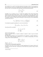
The control structure diagram of the continuous mixing technology system proposed by the
article is shown in Fig. 2. In which: The plant is a continuous mixing technology system;
Reference Model is the identification model; Adaptive Mechanism is the adaptive control block;
Compensation is the reciprocal block that compensates for uncertain components; SMC is a
sliding mode controller.

d (t )

xd

u smc

SMC

u

x

Plant

u ad
Reference
Model

Compensation

xm
e

fˆ ( x ) dˆ ( t )
Adaptation
Mechanism

Fig. 2. The control structure diagram of the continuous mixing technology system

Plant with the model (11) will follow the desired signal vector xd if the control law u is

selected in the form:
u = u smc + uad ,
(12)
where u smc is the sliding mode control law; uad is an adaptive control law.
3.1. Synthesis of the adaptive control law
We rewrite equation (11) as:
x = Ax + Bu + If  ,

(13)

where f = f ( x ) + d ( t ) =  f 1 , f  2  ; I is identity matrix. Substitute (12) into (13):
x = Ax + Bu smc + Bu ad + If .
From (14), we can see that uncertain elements will be compensated with the condition:
Bu ad + If = 0 .
To satisfy equation (15), we choose: u ad = −Hf ,
T

where H = BT BBT 

−1

is the gain matrix; det ( BBT )  0 .

(14)
(15)
(16)

In order to synthesize the control law (16), it is necessary to identify the nonlinear components

f ( x ) and the external disturbance d ( t ) present in f  .


The identification model for uncertain parameters in (11) can be written:
xm = Ax + Bu + fˆ ( x ) + dˆ ( t ) ,
where xm =  xm1 , xm 2 

T

(17)

is state vector of the model; fˆ ( x ) =  fˆ1 ( x ) , fˆ2 ( x ) 

T

is the estimated

vector of f ( x ) ; dˆ ( t ) =  dˆ1 ( t ) , dˆ2 ( t )  is the estimated vector of d ( t ) .
T

From (11) and (17), we have: e = Ae + f ( x ) + d ( t ) ,
where: e = x − xm ,


(19)

f ( x ) = f ( x ) − fˆ ( x )
82

(18)
(20)


d ( t ) = d ( t ) − dˆ ( t )

(21)

Email:


TNU Journal of Science and Technology

227(07): 79 - 87

Identification progress will be converging when f ( x ) → 0 , d ( t ) → 0 . With the assumption A
is a Hurwitz matrix, so e → 0 , and (18) is stability.
With f ( x ) is a smooth function vector, by using a RBF neural network for the approximation
[15]. The elements of f ( x ) can be written:
L

f i ( x ) =  wij*ij ( x ) +  i ,

(22)

j =1

i = 1, 2 ; j = 1, L where L is number of basis function with a large enough number to guarantee

the error  i   im ,  im = const ; wij* = const is the ideal weights. The basis functions are selected by
the following form:

(


ij ( x ) = exp x − cij

2

)

2 ij2 , i = 1, 2 , j = 1, L ,

(23)

where cij are the position of the center of the basis functions ij ( x ) , and  ij are the standard
deviation of the basis functions.
The estimated vector fˆ ( x ) is defined by (23) with adjusted weights wˆ ij :
L

fˆi ( x ) =  wˆ ijij ( x ) , i = 1, 2 , j = 1, L .

(24)

j =1

Training of the RBF neural network is implemented by adjustment of the weights wˆ ij in
comparison with the ideal weights wij* :
wij = wij* − wˆ ij .
(25)
From (22), (24), with attention to (25), we have:
fi ( x ) = fˆi ( x ) +  i

L


f (x) =  wijij ( x ) +  i .

→

(26)

j =1

For equations (18), the Lyapunov function is selected as follows:
2

L

2

V = eT Pe +  wij2 +  d i2 .
i =1 j =1

(27)

i =1

where P is a positive definite symmetric matrix. The equations (18) will be stable if the
derivative (27) V  0 . Take the derivative of both sides of (27):
2

L

2


V = ePe + eT Pe + 2 wij wij + 2 d i d i .
i =1 j =1

(28)

i =1

Substitute (18) into (28):
V = eT ( AT P + PA ) e + 2eT Pf ( x ) + 2eT Pd ( t ) + 2 wij wij + 2 d i d i .
2

L

i =1 j =1

2

i =1

(29)

From (29) and (26), we have:


 L



  w1 jij ( x )  2 L
2

j =1


T
T
T
T



V = e ( A P + PA ) e + 2e Pε + 2 e P L
+  wij wij  + 2  eT Pd ( t ) + 2 di di  .



 i =1 j =1
i =1




  w2 jij ( x ) 
 j =1



The condition for V  0 is as follows:

eT ( AT P + PA ) e + 2eT Pε  0 ;




83

(30)

(31)

Email:


TNU Journal of Science and Technology

227(07): 79 - 87



 L



  w1 jij ( x )  2 L
j =1

+
2  eT P  L
w
w
ij ij  = 0



 
i =1 j =1


  w2 jij ( x ) 
j
=
1





(32)

2


2  eT Pd ( t ) + 2 di di  = 0
i =1



(33)
2

Transform the left side of the inequality (31): −eT Qe + 2  i Pi e  0 ,

(34)


i =1

Q = − ( AT P + PA ) , Pi is the i -th row of the matrix P .

Using inequality transformations [16], the equation (31) can be written:
2

2

−eT Qe + 2  i Pi e  −rmin (Q) e + 2  i Pi e  0 ,
2

i =1

(35)

i =1

rmin (Q) is the smallest eigenvalue of the matrix Q .

Thus, to satisfy the inequality (31) from (35), we must have:
2

e  2  i Pi / rmin (Q) .

(36)

i =1


Solving equations (32), (33), we have:
wij = −Pi eij ( x ) , i = 1, 2 , j = 1,...L ;

(37)

di = −Pi e , i = 1, 2 .

(38)

If simultaneous (36-38) is satisfied, then V  0 , so the system (18) is stable. The stability
domain of (18) defined at (36) is the entire state space except the neighborhood of the origin. The
stability domain of (18) defined at (36) is the entire state space except for the neighborhood of
the origin. The radius of this region depends on the approximate error of the RBF neural network,
where  i is arbitrarily tiny and can be ignored. Thus, the stability domain is the entire state space
except for the origin region with a radius close to zero.
With the identification results (24), (37), (38), we replace f  with fˆ as follows:
fˆ = fˆ ( x ) + dˆ ( t ) =  fˆ1 , fˆ 2  .


T

(39)

u ad = − Hfˆ ,
The control law uad (16) is rewritten as follows:
then (14) becomes:
x = Ax + Bu smc .
For (41), the control law is synthesized using the sliding mode control method.

(40)

(41)

3.2. Synthesis of the sliding mode control law
The error vector between the state vector x and the desired state vector xd :
x = x − xd → x = x − xd .
Substitute (42) into (41):
x = Ax + Bu smc + Ax d − x d .
For (43), the hyper sliding surface is chosen as follows [17]: s = Cx ,
T
where C is the parameter matrix of hyper sliding surface, det(CB)  0 , s =  s1 , s2  .
The next problem is defining u smc , which ensures system (43) movement towards the
sliding surface (44) and keeps it there.
u s
u eq

The control signal u smc can be written by: u smc = 



84

khi

s0

khi

s=0

,


(42)
(43)
(44)
hyper

(45)

Email:


TNU Journal of Science and Technology

227(07): 79 - 87

u s is the control signal that moves the system (43) towards the hyper sliding surface (44); u eq

is the equivalent control signal that keeps the system (43) on the hyper sliding surface (44).
The equation (45) can be rewritten as: u smc = ueq + u s .
s = Cx = 0 .
u eq is defined in [17]:

(46)
(47)

ueq = − CB CAx + CAx d − Cx d  .
From (43) and (47), we have:
(48)
Next, we define the control signal u s that moves the system (43) towards the hyper sliding
surface (44). For the hyper sliding surface (44), the Lyapunov function can be selected by:

−1

1 T
s s.
2

V =

(49)

Condition for the existence of slip mode can be written: V = sT s  0 .
Substitute (43) and (46) into (50), with attention to (47), (48), we have:
V = sT C ( Ax + Bu smc + Ax d − x d ) + CBu s   0 .

(50)
(51)

The inequality (51) is equivalent to: s CBu s   0 .
T

(52)

To satisfy (50) from (52), we have: u s = − CB   sgn ( s1 ) ,  sgn ( s2 )  ,
−1

T

(53)

 is a small positive coefficient.

Substitute (48) and (53) into (45), we have:
u smc

− CB −1  sgn ( s ) ,  sgn ( s ) T khi s  0
1
2 


.
=
−1
− CB  CAx + CAx d − Cx d  khi s = 0

(54)

Finally, the control signals (40) and (54) are used for (11). Thus, the paper has synthesized the
control law for continuous mixing technology.
4. Results and discussion
Continuous mixing technology is described in (6) with parameters shown in Table 1 [10], [11].
Table 1. Continuous mixing technology parameters and nominal values [10]
Parameter
c1

c2
k1
k2

Meaning
Concentration in the inlet flow q1
Concentration in the inlet flow q2

Valve constant

Nominal Value
24.9 kmol/m3

Kinetic constant

1.0 mol2/m6s

0.1 kmol/m3
0.2 m1/2/s

Perform Taylor expansion of equation (6) at the equilibrium point

( h , c
0

30

 ,  q10 , q20 
T

T

)

( x0 , u0 ) =

with h0 = 1.0 m, c30 = 12.15 kmol/m3, q10 = 0.1 m/s, q20 = 0.1 m/s. The


matrices (9), (10) are obtained as follows:
0 
 −0.1
A=
,
−
0.07
−
0.195



1 
 1
B=
.
12.75
−
12.05



(55)

(56)

Nonlinear function vectors and disturbance vectors in (11) are defined as follows:
0.025 x12 − 0.0125 x13 
f (x) = 
,

2 
 0, 2 x1 x1 + 0, 001x2 

(57)

0


d (t ) = 
.
0,
2sin
0.05
t
+
0,
25cos(0,
03
t
)
(
)



(58)

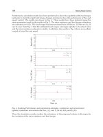
Simulations are implemented on the Matlab environment for the plant (11) using the
controller (12). The results of the identification of nonlinear components and external disturbance
T

f = f ( x ) + d ( t ) =  f 1 , f  2  using algorithms (24), (37), (38) are shown in Fig. 3.



85

Email:


TNU Journal of Science and Technology

227(07): 79 - 87

Fig 3. The identification vectors fˆ .

The simulation results in Fig. 3 show that the algorithm to identify the components of change
in plant kinematics has worked properly.
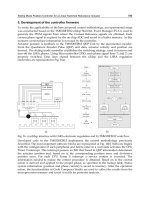
The results of the control law u ad (40) to compensate for the nonlinear component and the
external disturbance are expressed through the error ec = ec1 , ec 2  between the actual plant (11)
and the linear kinematic (41). The simulation results are shown in Fig. 4.
T

Fig 4. The error between (11) and linear model (41)

The simulation results in Fig. 4 show that the control law u ad (40) has compensated for the
nonlinear components and external disturbance in the plant kinematics with the offset error
asymptotically zero.
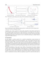
The results of tracking the state vectors of the system with the desired signal vector
T
xd = 1.0 12.15 using the sliding mode control law (54) are shown in Fig. 5.


Fig 5. Responses of the system for the desired signals xd = 1.0 12.15 .
T

From Fig. 5, it is shown that the system's response has to track to the desired signal h0 = 1.0 m
and c30 = 12.15 kmol/m3. Thus, with the controller (12), the continuous mixing technology control
system has created a desired concentration and volume solution with guaranteed control quality.
The simulation results have proved the correctness and effectiveness of the article's proposed
control law.
5. Conclusion
The article has synthesized the adaptive sliding mode control law for continuous mixing
technology. The law for identifying vectors of nonlinear functions and external disturbance has


86

Email:


TNU Journal of Science and Technology

227(07): 79 - 87

been built. From the identification results, building a compensation structure for their influence
on the system, the compensation error depends on the approximate error of the RBF neural
network. On the other hand, the RBF neural network can approximate with arbitrarily small
precision so that this error can be ignored. The control law of continuous mixing technology is
built on the principle of sliding mode control. When the adaptive algorithm converges, the
uncertainty elements are compensated so that the chattering effect in the sliding mode control law
is reduced to a minimum, which overcomes the limitation of the classical sliding mode control

method. The control system proposed by this paper is adaptable, resistant to interference, and has
good control quality. The simulation results once again proved the correctness and effectiveness
of the proposed method.
REFERENCES
[1] A. Jayachitra and R. Vinodha, “Genetic Algorithm Based PID Controller Tuning Approach for
Continuous Stirred Tank Reactor,” Advances in Artificial Intelligence, vol. 2014, 8 pages, 2014.
[2] M. A. Nekoui, M. A. Khameneh, and M. H. Kazemi, “Optimal design of PID controller for a CSTR
system using particle swarm optimization,” Proceedings of 14th International Power Electronics and
Motion Control Conference EPE-PEMC 2010, 2010, pp. T7-63-T7-66.
[3] K. Bingi, R. Ibrahim, M. N. Karsiti, and S. M. Hassan, “Fuzzy gain scheduled set-point weighted PID
controller for unstable CSTR systems,” 2017 IEEE International Conference on Signal and Image
Processing Applications (ICSIPA), 2017 pp. 289-293.
[4] M. Esfandyari, M. A. Fanaei, and H. Zohreie, “Adaptive fuzzy tuning of PID controllers,” Neural
Computing and Applications, vol. 23, pp. 19-28, 2013.
[5] A. Errachdi, I. Saad, and M. Benrejeb, “On-line identification of multivariable nonlinear system using
neural networks,” 2011 International Conference on Communications, Computing and Control
Applications (CCCA), 2011, pp. 1-5.
[6] R. S. M. N. Malar, S. Mani, and T. Thyagarajan, “Artificial neural networks based modeling and
control of continuous stirred tank reactor,” American Journal of Engineering and Applied Sciences,
vol. 2, no. 1, pp. 229-235, 2009.
[7] M. C. Colantonio, A. C. Desages, J. A. Romagnoli, and A. Palazoglu, “Nonlinear control of a CSTR:
disturbance rejection using sliding mode control,” Industrial & engineering chemistry research, vol.
34, no. 7, pp. 2383-2392, 1995.
[8] D. Zhao, Q. Zhu, and J. Dubbeldam, “Terminal sliding mode control for continuous stirred tank
reactor,” Chemical engineering research and design, vol. 94, pp. 266-274, 2015.
[9] O. Camacho and C. A. Smith, “Sliding mode control: an approach to regulate nonlinear chemical
processes,” ISA transactions, vol. 39, no. 2, pp. 205-218, 2000.
[10] S. R. Tofighi, F. Bayat, and F. Merrikh-Bayat, “Robust feedback linearization of an isothermal
continuous stirred tank reactor: H∞ mixed-sensitivity synthesis and DK-iteration approaches,”
Transactions of the Institute of Measurement and Control, vol. 39, no. 3, pp. 344-351, 2017.

[11] C. I. Pop, E. H. Dulf, and A. Mueller, “Robust feedback linearization control for reference tracking
and disturbance rejection in nonlinear systems,” Recent Advances in Robust Control - Novel
Approaches and Design Methods, 2011, pp. 273-290.
[12] M. R. Tailor and P. H. Bhathawala, “Linearization of nonlinear differential equation by Taylor’s series
expansion and use of Jacobian linearization process,” International Journal of Theoretical and Applied
Science, vol. 4, no. 1, pp. 36-38, 2011.
[13] Z. Vukic, Nonlinear control systems. CRC Press, 2003.
[14] J. J. E. Slotine and W. Li, Applied nonlinear control. Englewood Cliffs, NJ: Prentice Hall, 1991.
[15] N. E. Cotter, “The Stone - Weierstrass Theorem and Its Application to Neural Networks,” IEEE
Transaction on Neural Networks, vol. 1, no. 4, pp. 290-295, 1990.
[16] J. M. Ortega, Matrix Theory: A Second Course. Springer, 1987.
[17] V. I. Utkin, Sliding Modes in Control and Optimization. Springer - Verlag Berlin Heidelberg, 1992.



87

Email: