- Trang chủ >>
- Khoa Học Tự Nhiên >>
- Vật lý
Quantum mechanics large systems walter thirring
Bạn đang xem bản rút gọn của tài liệu. Xem và tải ngay bản đầy đủ của tài liệu tại đây (7.87 MB, 295 trang )
Walter Thirring
A Course
in Mathematical Physics
4
Quantum Mechanics
of Large Systems
Translated by Evans M. Harrell
Springer-Verlag New York Wien
Dr. Walter Thirring
Dr. Evans M. Harrell
Institute for Theoretical Physics
University of Vienna
Austria
The Johns Hopkins University
Baltimore, Maryland
U.S.A.
Translation of Lehrbuch der Mathematischen Physik
Band 4: Quantenmechanik grosser Systeme
Wien—New York: Springer-Verlag 1980
©
1980
by Springer-Verlag! Wien
ISBN 3-21 1-81604-6 Springer-Verlag Wien New York
ISBN 0-387-81604-6 Springer-Verlag New York Wien
Library of Congress Cataloging in Publication Data
Thirring, Walter E., 1927—
Quantum mechanics of large systems.
(A course in mathematical physics; 4)
Translation of: Quantenmechanik grosser Systeme.
Bibliography: p.
Includes index.
1. Statistical thermodynamics. 2. Statistical
mechanics. I. Title. U. Series: Thirring, Walter E..
Lehrbuch der mathematischen Physik.
English; 4.
530.l'Ss
82-19159
QC2O.T4513 vol.4 [QC3II.5]
.
With 39 Figures
© 1983 by Springer-Verlag New York Inc.
All rights reserved. No part of this book may be translated or reproduced in any form
without written permission from Springer-Verlag. 175 Fifth Avenue. New York.
New York 10010. U.S.A.
Typeset by Composition House Ltd Salisbury England
Printed and bound by R. R Donnelky & Sons. l-larrisonburg V A.
Printed in the United States of America
987654321
ISBN 0-387-81701-8
ISBN 3-211-81701-8
Springer-Verlag
York
Springer-Verlag Wien New York
www.pdfgrip.com
Preface
In this final volume I have tried to present the subject of statistical mechanics
in accordance with the basic principles of the series. The effort again entailed
following Gustav Mahler's maxim, "Tradition = Schlamperei" (i.e., filth)
and clearing away a large portion of this tradition-laden area. The result is a
book with little in common with most other books on the subject.
The ordinary perturbation—theoretic calculations are not very useful in
this field. Those methods have never led to propositions of much substance.
Even when perturbation series, which for the most part never converge, can
be given some asymptotic meaning, it cannot be determined how close the
nth order approximation comes to the exact result. Since analytic solutions
of nontrivial problems are beyond human capabilities, for better or worse
we must settle for sharp bounds on the quantities of interest, and can at most
strive to make the degree of accuracy satisfactory.
The last two decades have seen successful and beautiful treatments of many
fundamental issues—I have in mind the ordering of the states (2. 1), properties
of the entropy (2.2), noncommutative ergodic theory (3.1), the proof of the
existence of the thermodynamic functions (4.3), and the mathematical
analysis of Thomas-Fermi theory (4.1.2), which provides an understanding
of the stability of matter. The day is surely not far off when most of the
remaining holes in the conceptual structure of quantum statistical mechanics
will have been filled in and the questions that are not satisfactorily answered
today will be added to the list of achievements.
The successful completion of this course of mathematical physics in a.
reasonable time required the fortunate conjunction of several circumstances.
As with volume III, I had active support from several collaborators, and in
particular I am greatly obliged to B. Baumgartner, H. Narnhofer, A. Pflug,
and A. Wehrl. Countless other colleagues have helped indirectly by coping
www.pdfgrip.com
Vi
Prefac.
duties for me. The English rdition has again
1mm the cntical reading of B. Simon. The working con.ii the University of\ tenna were invaluable for thc completion of
hut not least, the fricLionless collaboration of Springer-Verlag
ii Vienna and my secretary and calligrapher F. Wagner enabled the books
to appear quickly and at a reasonable price.
I am aware that the uncompromising way of mathematical physics is
not the easiest. Yet I feel that it has been one of the greatest intellectual
gT
accomplishments of our era to cast the laws of Nature in a clear mathematical
form with rigorously deducible consequences. No amount of labor is too
high a price to have paid for this. Let me conclude by also acknowledging
and expressing my thanks to the reader who has borne with me to the end of
the course.
Walter Thirring
www.pdfgrip.com
Contents
Systems with Many Particles
1.1
1.2
1.3
1.4
2
Thermostatics
2.1
2.2
2.3
2.4
2.5
3
3.2
3.3
The Ordering of the States
The PropertIes of Entropy
The Microcanonical Ensemble
The Canonical Ensemble
The Grand Canonical Ensemble
4.2
4.3
20
29
45
57
73
103
115
144
rime-Evolution
The Equilibrium State
Stability and Passivity
Physical Systems
4.1
1
11
45
Thennodynamics
3.1
4
Equilibrium and Irreversibility
The Limit of an Infinite Number of Particles
Arbitrary Numbers of Particles in Fock Space
Representations with N =
144
173
191
209
Thomas-Fermi Theory
Cosmic Bodies
Normal Matter
Bibliography
209
242
256
279
Index
VII
www.pdfgrip.com
Systems with Many Particles
1.1 Equilibrium and Irreversibility
Macroscopic bodies cci in wi irreversible and deterministic manner
in con frost with rhe rerersible and indetermmisti character of the
of quantum physics. How can the apparent contradiction
systems of finitely many partic!es
,nforma(ion about the systems
a SU.e it
on the algebra (ci. (Ill: L.2.32)'; As our main goal is the study of e'.eryday
matter, our framework wilt oe that of nonrelativistic quantuu theory. For
the purposes of contrast, or of aiding intuition, we shall also have oecasion
to call upon classicai
where states
measures on phase space,
and extremal states are
measures. In either framework time-evolution
an automorphism a a, for a E d in the Heisenberg
picture. If desired, time
can alternatively, in the SchrOdinger
picture, he put upon the state: w . w,, such that
w(a1).
the algebra
is Abetian (classical mechanics), then the point of an extremal state moves
along a classical trajectory in phase-space.
In our earlier experience systems of N particle are so complex for large
N that it becomes impossible to reach precise, quantitative conclusions. It
turns out. however, that the theoretical analysis again simplifies in the limit
We have learned Lo describe
algebra .W ol observables.
N —+
Many properties become independent of the exact numbt'r of
particles and other detailed characteristics of the physical system, somewhat
in analogy to what happens in the central limit theorem of probability theory.
This may seem peculiar at first: we have always had d =
www.pdfgrip.com
2
1 Systems with Many Particles
separable Hubert space, and time-evolution was given by a unitary group
on .*'. What, then, appears so special about a many-particle system? Just
that the information contained in a pure state about a many-particle system
is so overwhelming that it would be too ambitious to employ the whole of
for the observables. Actual measurements could never be made on
more than a few observables, so
has to be cut down to size. For instance,
suppose that a device is only equipped to observe one particle at a time, and
is unable to detect correlations between particles. Then, rather than taking
the entire tensor product of the individual particles as the algebra of observables, it is reasonable to regard d as a single factor. Accordingly, many
states differing on
reduce to the same state when restricted to d. (The
classical situation is similar; the restriction of
fd3qi ...
w(x1,
d3p2 . ..
PN),
whole cylindrical regions of phase-space reduce to a single restricted
state.) As a consequence large portions of the space of states on
are
quite similar from the point of view of the reduced algebra .1. If, in the
Schrodinger picture, the state W, travels throughout the space of states, then
its restriction takes on a certain value with a very high probability, unless
so
prevented by some constants of the motion. This most probable state is called
the equilibrium state over d.
The irreversible tendency toward equilThrium has always aroused wonder,
especially as the basic equations of dynamics are invariant under reversal of
the motion (III: 3.3.18). We have even seen in classical mechanics that the
trajectory of any point on a compact energy surface returns arbitrarily close
to its initial position (1: 2.6.13). In quantum theory the Hamiltonian H of a
system confined to a finite volume has purely discrete spectrum. If and
denote the eigenvalues and eigenvectors of H, then the time-dependence
of an observable a is given by
w(a) =
—
3. k
where the state w is represented by the vector L if>. The state
is now
an almost-periodic function oft; if the sum is finite, and the are rationally
dependent, then it is actually strictly periodic. At any rate, to arbitrarily good
accuracy, w,(a) again becomes nearly w(a) after some sufficiently long delay.
The trouble is that the recurrence times are so unimaginably long that they
have no physical relevance. Suppose, for instance, that there are N distinct
energy differences
The recurrence time can then be estimated as follows.
The factors exp(iw3t) can be pictured as N clocks with hands moving at N
different rates. The question is how long it takes for a certain configuration
www.pdfgrip.com
1.1 Equilibrium and Irreversibility
3
of clock faces to reappear to within some angular accuracy
The con-
figuration in the space of angles has measure
so the recurrence time
is on the order of (&p/2irY
where the reciprocal angular velocity 1/co
is an average of the 1/wi. Even for just N = 10, 1/w = sec.. and
=
1/100, so that w, returns to w to within 1 oo accuracy, the recurrence time is
1020 sec., which is much longer than the age of the universe.
The approach to equilibrium is connected to a loss of information; to be
1
more precise, information does not get lost, but only less accessible. We
have seen that when the wave-packet of a free particle spreads (III: 3.3.3),
grows linearly with time, although the state remains pure and thus has
maximal information content. The observable with least deviation from the
mean is, however, not x(r) but x(0) x(t) — pi.
This behavior can be seen even in classical motion if a minimal spread of
the support of the probability distribution function in phase space is hypothesized to account for quantum effects. If, say, the initial probability density
p(p, q) is concentrated on a part of the energy shell {(q; p)1p1 p P2) and
is not pointlike. and it moves freely on a torus, then it eventually fills the
energy shell densely with a "fuzzy" distribution. Faster particles overtake
the slower ones, as bicycles racing in a stadium start packed closely together
but later draw apart and eventually spread around the whole track (see
Figure 1).
The ergodic hypothesis has figured importantly in the history of statistical
mechanics; it is the assumption that the trajectory of almost every point
winds densely around the energyshell in phase space, so that the time average
can be replaced with the average over the energy shell. On the one hand this
requires more than is necessary, since it suffices to fill a sufficiently typical
part of the energy shell, the average on which equals the average on the whole
shell for the reduced algebra of observables. On the other hand, although
macroscopic measurements last much longer than the collision time, they
last much less than the recurrence time, so one does not wait for the whole
energy shell to be sampled. We shall discuss examples in which the
equilibrium state is actually attained by the state in a reasonable time after
reduction to one particle.
A pictorial description of the situation is as follows. The information
about a subsystem (i.e., the opposite of the entropy, to be defined later) as a
function on the space of states of the total system Consists mainly of a plain
with few hills and still fewer mountains. The larger the total system, the
further apart the prominences. Even if a path begins on a peak. it soon
descends to the plain, and there is only the slightest probability that it will
ascend another mountain in any conceivable time. The time of descent to the
plain and the recurrence time are of completely different orders of magnitude.
It takes only the time corresponding physically to a few collisions to descepd
to a level near that of the plain, whereas the other mountains lie in the unfathomable distance. This means that equilibrium is reached long before the
immense recurrence time required to wind throughout the space of states;
www.pdfgrip.com
Systems with Many Particles
Figure 1
The motion of the density in phase space for a free particle on a torus.
www.pdfgrip.com
1.1
Equilibrium and Irreversibility
generally, a path soon reaches states that can not be distinguished from
equilibrium because of the limits of our measuring abilities. Of course, there
is still the question of how one happened, at the beginning, to be at the top
of the mountain, but that brings up the one of how the current state of the
universe came about and is outside the scope of this book.
Another puzzle is the apparent causal behaviof that classical thermodynamics prescribes for macroscopic bodies. According to the arguments
that have been advanced, one would rather suspect that the fluctuations of the
are increased by the loss of information. This is actually true for
microscopic variables like the positions and momenta of individual particles.
However, if only the so-called macroscopic observables are considered, that
is, roughly what was accessible to the more primitive experimental arts of an
earlier epoch. then deterministic features arise. Their origin is simply that
statistically independent quantities are being averaged: if a =
aj,
where
=
for i j, then
I
L
Thus 1w
(ajaiJ)
wf
\J.k
1
w(aJ)w(ak) I
—
J.tc
J
=
j=1
N 12, and for sufficiently large N the deviations from the average
are negligible. We shall learn that in the quantum-theoretical formalism such
an a approaches a multiple of the identity operator as N
x. The limiting
coefficient depends on the representation of the algebra.
Let us verify the phenomena described above in two explicitly soluble
models. Of necessity they will lack some of the complications arising in
reality, but they exhibit the important features. They are embryonic forms
of systems of fermions and bosons.
The Chain of Spins (1.1.1)
Let the algebra of observables'of the total system be generated by
j = 1,..., N, where each is a copy of the usual Pauli matrices Instead
and c±
of Cartesian components we use c
the commutation relations
± ia')/2, which satisfy
= ±ójk2(7k.
[a7,
=
(1.1.2)
The chain is closed by the identification of Gj+N with
and the Hamiltonian
that determines the time-evolution will be assumed to he of the form
•
H=B
N
N-i N
.
(1.1.3)
,i"i J=I
The physical meaning of this is that the spins are coupled with magnetic
j=1
moments p, to an, external magnetic field B, and in addition there is an
Ising like spin—spin interaction with the nth neighbor. The strength s(n) of
www.pdfgrip.com
I Systems with Many Partic!es
this interaction is a function that can be specified later, and the periodicity
allows us to assume
= 0 for n> N/2. If the contributions to H are
denoted as in
(1.1.4)
.
then the Hk commute with one another and with the o,. They are therefore
constant in time, and the time-evolution of & and a = (a+)* can
calculated easily from the relationship
f(cr)a
-I-
= a+f(a + 2),
which follows from (1.1.2). We find
=
= a(O) exP{21t[Biz& +
=
+
fl (cos 2t2(n) +
+
sin
2tE(n)
sin 2te(n)),
where a(t) = exp(iH)a exp( — iHi).
The time-evolution Consists of Larmor precession in the external field and
a kind of diffusion along the chain due to the spin—spin interaction. Suppose
that the state at r 0 is pure and has the form of a product, where the spins
have a 3-component s and
has phase
=
(n
=
5,
=
<Ci>.
(1.1.7)
Then
=
lv/1T? exp{i(; + 2tBpk))f2(O,
N'2
1(f) = fl(cos 2t.s(n) + is sin 2te(n)).
thenf (t) will generally
If N is finite, thenf is almost periodic, and if N =
(supposing that
tend to zero as t —.
tends to zero in such a way that
the infinite product makes sense). To make this more explicit, let us consider
the special case $ =
0
and c(n) =
If N =
cx,
then f satisfies
equation
f(r) = fJcos 2"r
Since
=
f is an entire function, this functional equation and the condition
f(0) =
I determinef uniquely—differentiate (1.1.9) to get the Taylor
off Since the function (sin t)/t satisfies (1.1.9), it equalsf. Hence, as N —*
www.pdfgrip.com
1.1 Equilibrium and Irreversibility
the expectation value of at approaches zero. For finite N it follows from
(1.1.9) that
= jicos 2"r
[sin
=
(1.1.10)
.
Therefore, as discussed earlier, the recurrence time
grows exponentially
with N, while the time it takes to reach equilibrium is independent of N.
To summarize, we have ascertained that for N = x the initially pure
stateofthealgebrareducedtoonespintendsasr
s to<a> s,<ct> = 0,
which corresponds to a mixture:
=
= Tr(pa).
Tr exp( —
s.
(1.1.11)
Even though the expectation values of the
go to zero, their fluctuations
remain nonzero, since
= (1 + ak). 2 is Constant. The average magnetization
(1.1.12)
MN(O =
k
= s. whereas
works differently. In the state (1.1.7) of our example,
2), provided either that the initial phases are disordered or
<Mi> is
a while because the
differ. The latter
that the
situation can in fact be undone by a sudden reversal of B, in the spin—echo
is irreversible, and
effect. If N = x, the diffusion caused by suitable
= 0. At ( = 0 the fluctuations are O(N12) and remain at
is calculated by multiplying together
this magnitude for all time: If
1.
two expressions of the form (1.1.6), then it should be recalled that a2
falls off sufficiently rapidly with ii, then the a2
However, if the function
terms make little difference for large k — k', and the argument given earlier
for the deviations of statistically independent quantities remains valid.
Chain of Oscillators (1.1.13)
Now represent the total system by positions and momenta q1
Pt
by
pj =
PN,such that
H
,and let the time-evolution be determined
+
(1.1.14)
This Hamiltonian contains interactions only between nearest neighbors. and
= q,, Pi+N =
the chain can be closed by the condition of periodicity
The masses and force constants have been set to 1, which amounts to measuring the time in units of the natural period of oscillation. The equations of
motion are
ci., =
+ q_1 —
=
www.pdfgrip.com
(1.1.15)
Systems with Many Particles
Wtth a periodic extension of the variables,
such
=
P,,,
that
—
they are put into the form
=
The variables
(1.1.17)
—
satisfy
=0.
Recall that the Bessel functions satisfy
the recursion formula
=
1)/2;as a consequence we see that the solution of the initial-value
—
problem is
=
(1.1.18)
Remarks (1.1.19)
z/v
-÷
1. Since I J,(z)
as
the sum over k in (1.1.18) converges
for, say, bounded
then (1.1.18) still holds provided that
2. If N <
=
3. Since the equations of motion are linear, the classical and quantum timeautomorphisms are identical.
4. There are still N constants of motion with the variables
2A'
1,..., N.
k
j
1
= 0, only N — I of the
With the auxiliary condition that
then
'2n+I = 0. If N =
constants are independent, and we find that
1k remains significant classically, provided that (4} E
in order to have a useful framework for discussing the questions that will
arise as in these two examples, it is convenient for technical reasons to make
use of the Weyl algebra (cf. (111, §3.1)). With one particle, the Wqyl algebra
consists of the operators W(r + is) = exp(i(pr + qs)), r, s E along with
their linear combinations and norm-limits. A state on the Weyl algebra is
uniquely characterized by the function E(r, s) <exp(i(pr + qs))>. We shall
only concern ourselves with coherent states (III: 3.1.13), which are of the
where I u> is a Gaussian function, the width of which deterform W(z')
I
mines the ratio between t.tp and Aq. Since
1
W(r + is)Iu> = exp[—
11
+
s2\1
—)j,
it follows that
In
—
E1,.,=0 =
=
www.pdfgrip.com
d2
In
1
=
Equihhrium and
9
The expectation value in the more general state W(z')lu> can be calculated
according to (III: 3.1.2; 1) as
W(:)I W(:' in; = (n.j W( — :)l'V(z) W(:"t a>
=
W(z)lu>
= expi—
—
+ i(rs -- r's)1. (1.1.20)
-.
i
L
Thus. the quantities
and &j are the same as wnh a>. but the
values of p and q
now and — r'.
of the
Let us return to the issue of how the
to a subsystem evolves in time. The operators
+
describe the momentum of a single particle and
position
neighbor. are useful to this end. Since
system. A state characterized by
I,
state
'shich
its
they form a
=
+ '2n+
+
—•
can be regarded as the generalization of (1.1.20).
Remarks (1.1.22)
and ,as appropriate
and
for a Weyl system for several particles, yet the variables
I
0.
are not pairs of canonically conjugate variables, since
J
1. The exponent on the left is a linear combination of
Thus (1.1.21) is not simply the tensor product of coherent states of a tensor
product of Weyl systems.
2. The significance of (1.1.21) is once again that the variables
all have deviation w and expectation values (rcsp. 11w and —
With (1.1.21), the desired state on the one-particle system turns Out to be
+
E(r, s)
=
+
= exp
+
±
+
+
{_
—
+
+
+
www.pdfgrip.com
+
(Li .23)
1 Systems with Many Particles
The sums can be evaluated by recourse to the formulas
=
.J/4t)),
+/2t) =
j E 7L,
—
(1.1.24)
which are derived in Problem 2. As t —, cc, only the terms withj = 0 remain.
Moreover, it can be seen from the integral representations and the Riemann—
Lebesgue lemma that the contributions linear in the 'k go to zero as t —
In all, we get
(co +
=
!)(r2 + s2)].
(1.1.25)
Remarks (1.1.26)
1. The limiting state corresponds to the mixture E = Tr pW(z), p
exp[ —
+
3). As to
1,
coth = (co + l/w)/2 (Problem
exp{ —
÷
that is, for minimal mean-square deviation,
cc, and the
state becomes pure. With larger mean-square deviations,
to
I,
l/w)/2 > 1, the limiting state is a mixture.
2. Whereas at I = 0 the ratio of
is to2, they become equal as t —, cc,
i.e., their ratio, 1, becomes the one defined by H. This corresponds to equal
amounts of kinetic and potential energy.
3. The reason that the existence of the constants (1.1.19; 4) does not prevent
the onset of equilibrium is again the choice of the initial state. Of course,
equilibrium can not occur if the system starts off in an eigenstate of a
normal mode of oscillation.
(to +
these few remarks will serve as our first orientation to irreversible
phenomena. We have already studied an example of an irreversible phenomenon in volume H, the emission of light. It is always important to take the
limit N —* cc before t -. cc, as in a finite volume the light returns to the point
of emission, and the behavior is almost periodic rather than irreversible.
The next section will deal with how the energy is affected by the first limiting
process.
Problems (1.1.27)
1. Calculate the entropy S(t) = —Tr p(z) In p(t) for one spin, wherefis given by (1.1.9).
2. Calculate
and
-
J21,+
3. Show that the density matrix p has the property stated in (1.1.26; 1).
www.pdfgrip.com
1.2 The Limit of an Infinite Number of
II
Solutions (1.1.28)
1.
Since Tr p(r)
Ic(i)l, which
I. the density matrix is of the form p(f)
The eigenvalues of p(t) are
ri +
S(t)=
I — e(t)
c(1)
I
+
2
c(,). r Let e(i) =
± c(t). so
I
—
In
2
2
Because
we find cU)
and therefore c(t)
±
(I
Observe that/is not monotonic, and hence that S does not increase
moaotonicalh from 0 to its equilibrium '.alue.
Ii + s
/1 +
/1 —
1— x
-• Ink-- 2) + ——i—
Putting:
x÷y
2-
1)]
yields
+ t) =
I)]
(r
—
—
=
=
so
fAx
I)]
(
=
is
j
J,,(x)J,
the addition theorem of Schläfii and
Neumann. Putting v = —x and changingj to —j then yields
,(x)
and with F = x. there results
=
from
= J_A2x)
hich formulas (1.1.24) follow.
Tr
+
=
2n)]
and
4 Tr
—
—
—
'
+ q2)j
+
lead to the result.
1.2
The Limit of an Infinite Number of Particles
The first issues to confront for large systems are what happens to
x.
macroscopic properties like energy and colume as N
I.! were only caricatures of reality. We shall now
determine the physical properties of large bodies. The first question is how
The models examined
www.pdfgrip.com
12
1 Systems with Many Particles
the volume V has to vary as N —+
in order to ensure that the potential and
kinetic energies will be comparable in magnitude and that the interaction
between the particles is correctly accounted for. In particular, when are E
and V normal, extensive quantities proportional to N? In order to fix our
ideas, we shall pay particular attention to certain special cases, large atoms
andmacroscopic or cosmic objects. The dominant force is then electrostatic,
except that in cosmic matter gravity also
a decisive effect. Heuristic
arguments will sometimes be adduced in this section for guidanceãn finding
which quantities have limits as N —'
in these systems.
Free Particles (1.2.1)
We begin with a consideration of noninteracting particles confined to a box
of side R. The energy consists of the quantum-mechanical zero-point energy
plus a thermal component proportional to the temperature T. As we are
only interested in the dependence on N for large N, we set h = k = m 1.
As explained in (111: 1.2.11) the zero-point energy of a system of fermions is
about RN113, since the volume available
per fermion is only R3/N. We arrive at
where
is
E=
+
(1.2.2)
If the two contributions are to remain comparable as N
and if T goes
as N' for some power t, then R must be N"3 t12, and
will tend
to a limiting value. The type of interaction will determine the value of t at
which the limit is nontrivial and thus of physical interest. For this to happen
the kinetic and potential energies have to remain of the same order of
magnitude.
Bosons do not have the solitary temperament, so
R. The energy is then on the order of
E
=
+
may be set equal to
(1.2.3)
If the two cuntributions are to have the same dependence on N and we make
N - ti2 and E
T N', then R
N'
If it is insisted that T remain
constant and R
then E N, but the zero-point energy drops below
the thermal energy. The exact calculation for free bosons in fact reveals that,
with a fixed particle density and below a critical temperature, a certain
0 of the particles are to be found in the ground state with
fraction
This makes this
E0
N"3, and thus N may be replaced with (1 —
usual limit also nontrivial.
www.pdfgrip.com
1.2 The Limit of an lnflnite Number of Particles
Large Atoms (1.2.4)
The Hamihonian of a large atom (with e2 =
H=
1)
is
12
I
+
—
—
(1.2.5)
which can, if one wishes, be confined in a box. Recall that in volume 11! we
figured out that if T = 0 and Z =
the energy is about
—
which has a minimum about
for R N 13 Therefore, in the limit
N
we should expect to set t =
In §4.1 it will not only be proved that
these limits converge, but even that the Thomas-Fermi theory becomes
exact in that limit. The problem can thus be solved in the limit N -.
though the solution is not suitable for a direct numerical comparison of
theory and experiment. Since there are corrections of about N - If 10%
accuracy can not be expected for N
On the other hanô, relativistic
effects become significant when t'i
102. The kinetic energy is then
N4' 3/R
and if Ze2 > 1 the energy is no longer bounded below. Hence the picture
that emerges of a large atom is only an idealization, but at least one with
many instructive aspects.
Systems of bosons depend on N in a different way. They all settle into the
ground state, and with Z N the radius goes as N and the energy as N3.
The limits of EN and N3p(xN) would be expected to exist, where p is the
one-particle density distribution, For thermal effects to remain significant,
T must be chosen —N2. This problem is mostly of academic interest, and the
convergence of the quantities mentioned above has not yet been proved.
Jellium (1.2.6)
Like an atom, jellium consists of particles repelling one another with a
Coulomb force and immersed in the field of an external charge distribution.
The difference is that the charge distribution is not concentrated at a point,
but rather homogeneously spread with density through a box A (A will
also sometimes denote the volume of A). It can be regarded as a model of
highly compressed matter. with the homogeneous background charge
coming from fast-moving electrons, and the particles with explicit coordinates
being the nuclei. It is nevertheless often used to describe electrons in a metal,
although it is rather far-fetched to speak of the assemblage of ions as a
homogeneous background. The Hamiltonian is
= N
U(xj + fd3xu(x). (1.2.7)
+
—
—
d3x = N.
where U(x) =
d3x'1 Ix — xj. For the system to be neutral,
The electrostatic energy of the background has been added in so that the
www.pdfgrip.com
14
1
Systems with Many Particles
potential energy will remain bounded below, by N(RN- 1/3)_ I, where R
is the linear dimension of A. The proof of this relies on the well-known fact
of electrostatics that the Coulomb repulsion.of two homogeneously charged
spheres is less than or equal to that of two point charges at their centers—the
inequality occurs when they overlap. Now imagine blowing the charged
particles up to homogeneously charged spheres of radius a, and let
I4ira3\2
d3xd3x'
5Jx—xiIa
f4ira\
(—c--I
\
/
=
X — X,
(1.2.8)
1
I
'Ix—xda
Then If may be written in the form
H=
i.j=1
i=1
2
p
—
U(x1))—
U11(a) +
i—I
Contribution
—
—
i
(1.2.9)
is positive, since it is of the form
dx dx'
p(x)p(x'),
J x—
and I/c has a positive Fourier transform. It is easy to show (Problem 1) that
equality holding provided that all the spheres lie within
fi
A, and)' = (N/2X6/5a), the self-energy of homogeneously charged spheres.
+ (3/5a)) is
As discussed earlier, ö 0. The lower bound —
which is precisely the radius at which the
optimized at a =
sum of the volumes of the spheres equals that of A. This coniputation leads
to the
Lower Bound for the Energy (1.2.10)
Remarks (1.2. 11)
1. Nothing has yet been assumed about the shape of A or the statistics of the
particles. In particular, if A is spherical, then by Problem 2,
U(x1) +
—
where equality holds if
5
d3xU(x)
E A for all I.
www.pdfgrip.com
1x112 —
15
1.2 The Limit ofan Infinite Number of Particles
2. Despite its great generality, the numerical accuracy of the bound (1.2.10)
is surprisingly good. If x1 are the sites of a simple, face-centered, or bodycentered cubic lattice, computer studies have been made of the limit as
N
x' of the potential energy over Nr ',yielding respectively the values
—0.880, —0.895, and —0.896 [3].
Lower bounds for H depending on the particle statistics may be derived
from (1.2.10). The energy of free fermions is. as seen earlier, —N5 31R2
Nr 2 and with the aid of the more precise proportionality factor,
H N( 1.1
2
— 0.9r') —
N
for all
e R+
(1.2.12)
for spin-i particles. Even if the volume and consequently r5 are treated 'as
variables, the resultant lower bound is N. We shall discover later that with
no more than first-order perturbation theory we can obtain an upper bound
not much different from (1.2.12): the Pauli exclusion principle makes the
electrons stay at a distance r, apart, and this correlation imitates the energetically favorable configurations of (1.2.11: 2). Since the minimizing radius
N 13, so the exponent
N and R
r3 does not depend on N, in this model E
t of (1.2.1) equals zero.
A very different picture emerges of bosons. With the kinetic energy (1.2.3)
we find, ignoring precise coefficients, that
N1'3
H —i—
r;
The minimizing
is
N
r
— —.
N23, and so E —
(1.2.13)
N5
Remarks (1.2.14)
1.
2.
displays the correct
It is uncertain whether the lower bound
dependence on N. Upper hounds obtained with trial functions include
more kinetic energy since the particles have to be correlated in order to
attain a sufficienLly negative potential energy. Until recently it was only
possible to show that E < —eN7'5 [1].
If the background charge is concentrated at discrete points of a lattice.
then trial functions can be thought up that show E < —eN5'3, and thus
in this case the energy in fact goes as N5 [2].
3. So far only the electrostatic energy has been accommodated m the backIf the background
ground. and minimized according to the density
consists of electrons, then its zero-point energy must also be calculated.
In a jellium of deuterium atoms, which are bosons, the energy turns out
to be N: The background density prevents them from collapsing, and
for fixed r5 (1.2.13) is on the order of N.
www.pdfgrip.com
Systems with Many Particles
I
Real Matter (1.2.15)
Real matter consists of positive and negative point-particles interacting with
a Coulomb force, so
H =
±
m1
L
(1.2.16)
-
—
,>,
for particles confined to a box of volume A
R3. We shall often particularize
to the situation wherein all negative particles are identical with m = lel =
and all positive particles are identical with mass M and charge Z. Provided
that Z is not so large that relativistic effects become significant, (1.2.16) gives
a reasonably accurate description of ordinary matter. We Therefore expect
to find that E
N113.
—N for R
The proof of this fact, known as the "stability of matter," has to be deferred
to §4.3. At this point we shall make do with several
Remarks (1.2.17)
1. Roughly speaking, the difficulty is that the double sum for the kinetic
energy contains —. N2 terms, so many cancellations are needed for the
result to be only N. If, as in the gravitating system to be described
shortly (1.2.19), all the contributions are of like sign, then cancellations
certainly do not occur. Similarly, if the total charge Q L e is N213 +
N113, the
and the system is restricted to a region of linear dimension R
energy fails to be extensive. The electrostatic energy Q2/R is N only if
Q
N213.
N if all the
particles are bosons. To prove this, rewrite (1.2.16) (with M = Z = 1) as
2. Even requiring that Q = 0 will not guarantee that
H=
i=1
2
L
i=1
I El
+ L lxr —xfl1 + Lix: —xfl-'
—xL',
(1.2.18)
where N + = N for a neutral system. Now take the expectation value in
are the trial functions that led to
a state with 'P + 0 'P , where
E
— N"5 for Bose-jelli.um. Although the particles are correlated, the
charge density is homogeneous, as for instance
=
U(x)
U(xr) -The last term in (1.2.28) is therefore equivalent to —
d3xU(x), and there results the sum of the energies of the positive
+
and negative Bose-jellia. The expectation value is consequently about
— N"5, which is an upper bound to the energy by the mm—max principle
www.pdfgrip.com
12 The Limit of an tnfinite Number of Particles
(III: 3.5.21). This "instability." which corresponds to the ground-state
energy being nonextensive and the spatial contraction of many-particle
aggregates of charged bosons, does not imply that individual atoms conof oppositely charged bosons would be unstable. A single, nonrelativistic atom of He4 with its electrons subjected to Bose statistics (but
with their original mass and charge) would have the same ground-state
energy as real He4, since the two-particle ground-state wave-function is
symmetric in the spatial coordinates. The lesson here is that experience
with two-electron molecules is not a trustworthy guide to the problem of
the stability of matter: Since the Pauli exclusion principle makes no
difference, the two electrons might just as well be bosons, but a system of
many bosons would be unstable, whereas a many-fermion system is
stable.
3. Since He3 is just as stablc as He4. stability is not a matter of the type of
statistics of one of the kinds of charge-carrier. Moreover, the relevant
energy is always measured in Rydbergs, using the electronic mass, so
matter should remain stable even in the limit of infinite nuclear masses.
4. It could be argued heuristically that the potential energy should go as
—N4'3R 1, since each charge sees an opposite charge at a distance
RN - "i. while charges further away should be screened. If this is added to
the kinetic energy N5 3R - of fermions or NR - 2 of bosons, the minimum
N"3 or —N513 at R N"3.
is respectively —N at R
1/Ax, so the system
5. In relativistic dynamics the kinetic energy is
is softer. The heuristic arguments would evaluate the total energy of
bosons as N/R — e2N413/R, which is unbounded below when N is
sufficiently large. Whereas nonrelativistic energies are always semibounded
for any fixed N, it may happen that the relativistic energy goes to — for
sufficiently large, but still finite, values of N.
6. The instability of a Coulomb system of bosons has nothing to do with the
long range of the l/r potential, but comes from its short-range features. If
the singularity is chopped off by changing the potential to V(x) =
the system of bosons also becomes stable: Since the
exp( —
Fourier transform of V is
(1 —
—
V(k)
with
=
e,
=
0)
1k12(1k12+
we find that
1N
2
V
—
Xj)
1
—
=
(2ir)
>
H is bounded below by — cN. It could be argued that nuclei have a
form factor, and that if jt is taken as the reciprocal of the nuclear radius,
so
www.pdfgrip.com
18
1
Systems with Many Particles
then V would be a more realistic potential than 1/r. This would lead to a
simple proof of stability, but it misses the real point. Since the Rydberg,
which is measured in electronvolts (eV), is determined by the mass of the
electron, it is the kinetic energy of the electrons rather than the size of the I
nuclei that matters most for stability. The lower bound from the size of
the nuclei alone would be — N MeV.
Cosmic Bodies (1.2. 19)
The hr potentials in an object with gravitationally interacting particles are
all attractive, so the situation is drastically different. The ground state of the
Hamiltonian
HG.=
(1.2.20)
goes as — N713 for fermions. By the now familiar argument, E
N513/R2 —
N - "i. This can
N2/R, which has its minimum value
— N713 for R
easily be translated into an exact upper bound by the use of trial functions
Lower bounds are harder to come by, since energetically
localized in
more favorable possibilities have to be ruled out. In this case there is an easier
way: Write
N
/i12
LI —
V VI
—
-
i-11i_.
N
f l=t
that each h, is the Hamiltonian of an atom with electrons having no
1=1
so
"N — I'
\
— ) 1*1 —
Coulomb repulsion. Particle number i stands for the atomic nucleus, as it has
no kinetic energy, and the others are electrons, with mass N — 1 and potential
—
— x31 1/2. According to (III: 4.5.15) it follows that h, —cN4'3, and
indeed the result is a
Bmmd for the Energy of Gravitating Fermlons (1.2.22)
HG> —cN713,
c = 0(1).
Remarks (1.2.23)
1. Fermi statistics were not fully taken into account, since we have only anti-
symmetrized with respect to N — 1 particles when filling the energy
levels. Since complete antisymnietnzation restricts the set of admissible
functions further, (1.2.22) is at any rate a lower bound.
2. The limit as N -. in this case exists with the scaling behavior t = of
(1.2.1), as in (1.2.4). This does not mean that the limit with t = fails to
exist for ordinary matter, but only that it is trivial. The potential energy
goes to zero and the particles remain free.
3. If the particles are bosons, then they can all be put into the ground state,
and E —N3. The radius of the ground state then goes as N'.
4. The Hamiltonian (1.2.20) was for the discussion of electrically neutral
particles;. if they are instead
charged, then K must be replaced with
www.pdfgrip.com
1.2 The Limit of an infinite Number of Particles
19
DC —
If we bear normal matter in mind, the gravitational force comes
from the protonic mass, and in units where the mass of the proton is 1,
iqe2
10 36• Inequality (1.2.22) then a fortiori provides a lower bound,
since
IC
i>j lxi — XjI
—
X1 — X,I
— 2C1C2N7"3
The number of particles determines which N-dependence dominates.
Gravity begins to win out when N (e2/K)312 iOfl, which is about the
mass of Jupiter, and the energies of larger heavenly bodies are controlled
mainly by gravitation. A concrete
is that the atoms get
squashed and turn into a plasma of nuclei and electrons. This inequality
provides a more rigorous foundation for the heuristic considerations of
(II: 4.5.1).
We shall see in §4.2 that the system (1.2.20) can be solved in the limit
co, as the Thomas-Fermi theory becomes exact. Thomas—Fermi theory'
provides an idealization of stars, various corrections again being needed to
make it realistic. In particular, if N
10" relativistic effects become important. As with atoms with Z> 137, the Hamiltonian is unbounded below,
N -+
which leads to a catastrophe. Nonetheless, Thomas—Fermi theory reflects the
thermodynamic properties of stars rather well.
This section concludes with Table 1 displaying the many possibilities:
Table I
The N-dependence of the kinetic energy K and the potential energy V when
N is large.
electric
K
V
Rmin
IBose
N/R2
—AV"3/R
N"3
IFermi
N513/R2
—N413fR
N113
—N
N/R2
—N2/R
N'
—N3
N513/R2
—N2/R
N113
—N213
N/R
— N413/R
0
—
N413/R
—
0
or co
or 0
— N2/R
0
—
N2/R
0
—
Nonrelativistic
{ gravitational iFermi
(Bose
electric
Fermi
N"3/R
t
Relativistic
{ gravitational
I Bose
}
N/R
N43/R
—
N513
—
t If Rmj,, tends to + co more rapidly than Nt13, then the kinetic energy per particle,
N113/R, becomes arbitrarily small, eventually 4 m, and the system is nonrelativistic.
Which energy breaks the staleHence Rm,n certainly can not increase faster than N
mate depends on the strength of the charge. If Z < 137, the kinetic energy wins out, and
if Z> 137, the potential energy wins out.
www.pdfgrip.com
20
1
Systems with Many Particles
Problems (1.2.24)
1. Calculate the fi and y of (1.2.9).
2. Verify
(1.2.11;
1).
Solutions (1.2.25)
v:f
= Jr2 dr dflr'2 dr'
—
r) +
—
rI)]
fri a
=
ff' r2 dr r'2 dr'(°<"r,
r)
+
2n
1
®(i—
=
p:f
I
— ,('I
lx'l/
xis.
The second integral equals 0, as can be seen by expanding Ix
—
harmonics. The first integral equals —(2xa2/5X4,ra3/3) if (x': Ix'(
otherwise greater than or equal to this.
2.
x'I' in spherical
a}
A, and is
—(3N/2R) + (N/2RX1x1I2/R2), equality holding for Ixjj
1.3 Arbitrary Numbers of Particles in Fock Space
The properties of large systems should not depend on the exact
number of particles, so it is convenient to use &representalion with a
variable number of particles.
We are used to dealing with atomic systems on
the n-particle Hilbert
space. As it is impossible to count the particles in a large system, it is convenient to regard the number N of particles as an observable capable of
assuming various values. Accordingly, we shall study Fock space
(1.3.1)
as the foundation for later analysis. The space
is one-dimensional and
spanned by the vacuum vector
If the particles under consideration are
either all bosons or all fermions, then *',, is either the n-fold symmetric or
which
totally antisymmetric tensor product of
= L2(R3, d3x) with
www.pdfgrip.com


![Lecture notes on c algebras and quantum mechanics [jnl article] n lamdsman](https://media.store123doc.com/images/document/14/rc/rt/medium_6PjfnHupCQ.jpg)

![Matrix quantum mechanics and 2 d string theory [thesis] s alexandrov](https://media.store123doc.com/images/document/14/rc/ya/medium_8kAdgQLKd0.jpg)