- Trang chủ >>
- Khoa Học Tự Nhiên >>
- Vật lý
Principles of mechanics
Bạn đang xem bản rút gọn của tài liệu. Xem và tải ngay bản đầy đủ của tài liệu tại đây (11.64 MB, 179 trang )
Advances in Science, Technology & Innovation
IEREK Interdisciplinary Series for Sustainable Development
Salma Alrasheed
Principles
of Mechanics
Fundamental University Physics
www.dbooks.org
Advances in Science, Technology & Innovation
IEREK Interdisciplinary Series for Sustainable
Development
Editorial Board Members
Anna Laura Pisello, Department of Engineering, University of Perugia, Italy
Dean Hawkes, Cardiff University, UK
Hocine Bougdah, University for the Creative Arts, Farnham, UK
Federica Rosso, Sapienza University of Rome, Rome, Italy
Hassan Abdalla, University of East London, London, UK
Sofia-Natalia Boemi, Aristotle University of Thessaloniki, Greece
Nabil Mohareb, Beirut Arab University, Beirut, Lebanon
Saleh Mesbah Elkaffas, Arab Academy for Science, Technology, Egypt
Emmanuel Bozonnet, University of la Rochelle, La Rochelle, France
Gloria Pignatta, University of Perugia, Italy
Yasser Mahgoub, Qatar University, Qatar
Luciano De Bonis, University of Molise, Italy
Stella Kostopoulou, Regional and Tourism Development, University of Thessaloniki,
Thessaloniki, Greece
Biswajeet Pradhan, Faculty of Engineering and IT, University of Technology Sydney, Sydney,
Australia
Md. Abdul Mannan, Universiti Malaysia Sarawak, Malaysia
Chaham Alalouch, Sultan Qaboos University, Muscat, Oman
Iman O. Gawad, Helwan University, Egypt
Series Editor
Mourad Amer, Enrichment and Knowledge Exchange, International Experts for Research,
Cairo, Egypt
www.pdfgrip.com
Advances in Science, Technology & Innovation (ASTI) is a series of peer-reviewed books
based on the best studies on emerging research that redefines existing disciplinary boundaries
in science, technology and innovation (STI) in order to develop integrated concepts for
sustainable development. The series is mainly based on the best research papers from various
IEREK and other international conferences, and is intended to promote the creation and
development of viable solutions for a sustainable future and a positive societal transformation
with the help of integrated and innovative science-based approaches. Offering interdisciplinary
coverage, the series presents innovative approaches and highlights how they can best support
both the economic and sustainable development for the welfare of all societies. In particular,
the series includes conceptual and empirical contributions from different interrelated fields of
science, technology and innovation that focus on providing practical solutions to ensure food,
water and energy security. It also presents new case studies offering concrete examples of how
to resolve sustainable urbanization and environmental issues. The series is addressed to
professionals in research and teaching, consultancies and industry, and government and
international organizations. Published in collaboration with IEREK, the ASTI series will
acquaint readers with essential new studies in STI for sustainable development.
More information about this series at />
www.pdfgrip.com
www.dbooks.org
Salma Alrasheed
Principles of Mechanics
Fundamental University Physics
123
www.pdfgrip.com
Salma Alrasheed
Thuwal, Saudi Arabia
ISSN 2522-8714
ISSN 2522-8722 (electronic)
Advances in Science, Technology & Innovation
ISBN 978-3-030-15194-2
ISBN 978-3-030-15195-9 (eBook)
/>Library of Congress Control Number: 2019934801
© The Editor(s) (if applicable) and The Author(s) 2019. This book is an open access publication.
Open Access This book is licensed under the terms of the Creative Commons Attribution 4.0 International License
( which permits use, sharing, adaptation, distribution and reproduction in
any medium or format, as long as you give appropriate credit to the original author(s) and the source, provide a link to
the Creative Commons license and indicate if changes were made.
The images or other third party material in this book are included in the book’s Creative Commons license, unless
indicated otherwise in a credit line to the material. If material is not included in the book’s Creative Commons license
and your intended use is not permitted by statutory regulation or exceeds the permitted use, you will need to obtain
permission directly from the copyright holder.
The use of general descriptive names, registered names, trademarks, service marks, etc. in this publication does not
imply, even in the absence of a specific statement, that such names are exempt from the relevant protective laws and
regulations and therefore free for general use.
The publisher, the authors and the editors are safe to assume that the advice and information in this book are believed
to be true and accurate at the date of publication. Neither the publisher nor the authors or the editors give a warranty,
expressed or implied, with respect to the material contained herein or for any errors or omissions that may have been
made. The publisher remains neutral with regard to jurisdictional claims in published maps and institutional
affiliations.
This Springer imprint is published by the registered company Springer Nature Switzerland AG.
The registered company address is: Gewerbestrasse 11, 6330 Cham, Switzerland
www.pdfgrip.com
www.dbooks.org
Preface
This book is aimed at taking the reader step by step through the beautiful concepts of
mechanics in a clear and detailed manner. Mechanics is considered to be the core of physics
and a deep understanding of the concepts is essential for all branches of physics. Many proofs
and examples are included to help the reader grasp the fundamentals fully, paving the way to
deal with more advanced topics. This book is useful for undergraduate students majoring in
physics or other science and engineering disciplines. It can also be used as a reference for more
advanced levels.
I would like to express my deep gratitude to my parents Abdulkareem Alrasheed and Mona
Alzamil for their encouragement and support. I am grateful to all of those who have contributed to this book and made its completion possible. In particular, I would like to thank
Khalid Alzamil, Dr. Laila Babsail, and Abbie Clifford for their efforts in revising the book. My
sincere thanks are also extended to Ardel Flavier and Rodolfo Rodriguez for their assistance in
creating the figures and illustrations. Finally to my daughter Layla, words can’t express my
appreciation to you.
Jeddah, Saudi Arabia
January 2019
Dr. Salma Alrasheed
v
www.pdfgrip.com
Contents
1
Units
1.1
1.2
1.3
1.4
1.5
1.6
.
.
.
.
.
.
.
.
.
.
.
.
.
.
.
.
.
.
.
.
.
.
.
.
.
.
.
.
.
.
.
.
.
.
.
.
.
.
.
.
.
.
.
.
.
.
.
.
.
.
.
.
.
.
.
.
.
.
.
.
.
.
.
.
.
.
.
.
.
.
.
.
.
.
.
.
.
.
.
.
.
.
.
.
.
.
.
.
.
.
.
.
.
.
.
.
.
.
.
.
.
.
.
.
.
.
.
.
.
.
.
.
.
.
.
.
.
.
.
.
.
.
.
.
.
.
.
.
.
.
.
.
.
.
.
.
.
.
.
.
.
.
.
.
.
.
.
.
.
.
.
.
.
.
.
.
.
.
.
.
.
.
.
.
.
.
.
.
.
.
.
.
.
.
.
.
.
.
.
.
.
.
.
.
.
.
.
.
.
.
.
.
.
.
.
.
.
.
.
.
.
.
.
.
.
.
.
.
.
.
.
.
.
.
.
.
1
1
1
2
2
3
3
3
3
4
4
4
5
5
5
5
5
6
7
7
8
11
11
12
12
12
13
2
Kinematics . . . . . . . . . . . . . . . . . . . . . . . . . . . . . . . . . . . . . . . . . . . .
2.1 Introduction . . . . . . . . . . . . . . . . . . . . . . . . . . . . . . . . . . . . . . .
2.2 Displacement, Velocity, and Acceleration . . . . . . . . . . . . . . . . .
2.2.1 Displacement . . . . . . . . . . . . . . . . . . . . . . . . . . . . . . . .
2.2.2 Average Speed . . . . . . . . . . . . . . . . . . . . . . . . . . . . . .
2.2.3 Velocity . . . . . . . . . . . . . . . . . . . . . . . . . . . . . . . . . . .
2.2.4 Speed . . . . . . . . . . . . . . . . . . . . . . . . . . . . . . . . . . . . .
2.2.5 Acceleration . . . . . . . . . . . . . . . . . . . . . . . . . . . . . . . .
2.3 Motion in Three Dimensions . . . . . . . . . . . . . . . . . . . . . . . . . . .
2.3.1 Normal and Tangential Components of Acceleration . . .
2.4 Some Applications . . . . . . . . . . . . . . . . . . . . . . . . . . . . . . . . . .
2.4.1 One-Dimensional Motion with Constant Acceleration . .
2.4.2 Free-Falling Objects . . . . . . . . . . . . . . . . . . . . . . . . . . .
2.4.3 Motion in Two Dimensions with Constant Acceleration .
.
.
.
.
.
.
.
.
.
.
.
.
.
.
.
.
.
.
.
.
.
.
.
.
.
.
.
.
.
.
.
.
.
.
.
.
.
.
.
.
.
.
.
.
.
.
.
.
.
.
.
.
.
.
.
.
.
.
.
.
.
.
.
.
.
.
.
.
.
.
.
.
.
.
.
.
.
.
.
.
.
.
.
.
.
.
.
.
.
.
.
.
.
.
.
.
.
.
17
17
17
17
17
18
18
18
20
21
23
23
25
27
and Vectors . . . . . . . . . . . . . . . . . . . . . . . . . .
Introduction . . . . . . . . . . . . . . . . . . . . . . . . . .
The SI Units . . . . . . . . . . . . . . . . . . . . . . . . .
Conversion Factors . . . . . . . . . . . . . . . . . . . . .
Dimension Analysis . . . . . . . . . . . . . . . . . . . .
Vectors . . . . . . . . . . . . . . . . . . . . . . . . . . . . .
Vector Algebra . . . . . . . . . . . . . . . . . . . . . . .
1.6.1 Equality of Two Vectors . . . . . . . . . .
1.6.2 Addition . . . . . . . . . . . . . . . . . . . . . .
1.6.3 Negative of a Vector . . . . . . . . . . . . .
1.6.4 The Zero Vector . . . . . . . . . . . . . . . .
1.6.5 Subtraction of Vectors . . . . . . . . . . . .
1.6.6 Multiplication of a Vector by a Scalar
1.6.7 Some Properties . . . . . . . . . . . . . . . . .
1.6.8 The Unit Vector . . . . . . . . . . . . . . . .
1.6.9 The Scalar (Dot) Product . . . . . . . . . .
1.6.10 The Vector (Cross) Product . . . . . . . .
1.7 Coordinate Systems . . . . . . . . . . . . . . . . . . . .
1.8 Vectors in Terms of Components . . . . . . . . . .
1.8.1 Rectangular Unit Vectors . . . . . . . . . .
1.8.2 Component Method . . . . . . . . . . . . . .
1.9 Derivatives of Vectors . . . . . . . . . . . . . . . . . .
1.9.1 Some Rules . . . . . . . . . . . . . . . . . . . .
1.9.2 Gradient, Divergence, and Curl . . . . .
1.10 Integrals of Vectors . . . . . . . . . . . . . . . . . . . .
1.10.1 Line Integrals . . . . . . . . . . . . . . . . . .
1.10.2 Independence of Path . . . . . . . . . . . . .
.
.
.
.
.
.
.
.
.
.
.
.
.
.
.
.
.
.
.
.
.
.
.
.
.
.
.
.
.
.
.
.
.
.
.
.
.
.
.
.
.
.
.
.
.
.
.
.
.
.
.
.
.
.
.
.
.
.
.
.
.
.
.
.
.
.
.
.
.
.
.
.
.
.
.
.
.
.
.
.
.
.
.
.
.
.
.
.
.
.
.
.
.
.
.
.
.
.
.
.
.
.
.
.
.
.
.
.
.
.
.
.
.
.
.
.
.
.
.
.
.
.
.
.
.
.
.
.
.
.
.
.
.
.
.
.
.
.
.
.
.
.
.
.
.
.
.
.
.
.
.
.
.
.
.
.
.
.
.
.
.
.
.
.
.
.
.
.
.
.
.
.
.
.
.
.
.
.
.
.
.
.
.
.
.
.
.
.
.
.
.
.
.
.
.
.
.
.
.
.
.
.
.
.
.
.
.
.
.
.
.
.
.
.
.
.
.
.
.
.
.
.
.
.
.
.
.
.
.
.
.
.
.
.
.
.
.
.
.
.
.
.
.
.
.
.
.
.
.
.
.
.
.
.
.
.
.
.
.
.
.
.
.
.
.
.
.
.
.
.
.
.
.
.
.
.
.
.
.
.
.
.
.
.
.
.
.
.
.
.
.
.
.
.
.
.
.
.
.
.
.
.
.
.
.
.
.
.
.
.
.
.
.
.
.
.
.
.
.
.
.
.
.
.
vii
www.pdfgrip.com
www.dbooks.org
viii
Contents
2.4.4 Projectile Motion . . . . . . . . . . . . .
2.4.5 Uniform Circular Motion . . . . . . .
2.4.6 Nonuniform Circular Motion . . . .
Relative Velocity . . . . . . . . . . . . . . . . . . .
Motion in a Plane Using Polar Coordinates
.
.
.
.
.
.
.
.
.
.
.
.
.
.
.
.
.
.
.
.
.
.
.
.
.
.
.
.
.
.
.
.
.
.
.
.
.
.
.
.
.
.
.
.
.
.
.
.
.
.
.
.
.
.
.
.
.
.
.
.
.
.
.
.
.
.
.
.
.
.
.
.
.
.
.
.
.
.
.
.
.
.
.
.
.
.
.
.
.
.
.
.
.
.
.
.
.
.
.
.
.
.
.
.
.
.
.
.
.
.
.
.
.
.
.
28
29
30
31
32
3
Newton’s Laws . . . . . . . . . . . . . . . . . . . . . . . . .
3.1 Introduction . . . . . . . . . . . . . . . . . . . . . . .
3.1.1 The Concept of Force . . . . . . . . .
3.1.2 The Fundamental Forces in Nature
3.2 Newton’s Laws . . . . . . . . . . . . . . . . . . . .
3.2.1 Newton’s First Law . . . . . . . . . . .
3.2.2 The Principle of Invariance . . . . .
3.2.3 Mass . . . . . . . . . . . . . . . . . . . . . .
3.2.4 Newton’s Second Law . . . . . . . . .
3.2.5 Newton’s Third Law . . . . . . . . . .
3.3 Some Particular Forces . . . . . . . . . . . . . . .
3.3.1 Weight . . . . . . . . . . . . . . . . . . . .
3.3.2 The Normal Force . . . . . . . . . . . .
3.3.3 Tension . . . . . . . . . . . . . . . . . . . .
3.3.4 Friction . . . . . . . . . . . . . . . . . . . .
3.3.5 The Drag Force . . . . . . . . . . . . . .
3.4 Applying Newton’s Laws . . . . . . . . . . . . .
3.4.1 Uniform Circular Motion . . . . . . .
3.4.2 Nonuniform Circular Motion . . . .
.
.
.
.
.
.
.
.
.
.
.
.
.
.
.
.
.
.
.
.
.
.
.
.
.
.
.
.
.
.
.
.
.
.
.
.
.
.
.
.
.
.
.
.
.
.
.
.
.
.
.
.
.
.
.
.
.
.
.
.
.
.
.
.
.
.
.
.
.
.
.
.
.
.
.
.
.
.
.
.
.
.
.
.
.
.
.
.
.
.
.
.
.
.
.
.
.
.
.
.
.
.
.
.
.
.
.
.
.
.
.
.
.
.
.
.
.
.
.
.
.
.
.
.
.
.
.
.
.
.
.
.
.
.
.
.
.
.
.
.
.
.
.
.
.
.
.
.
.
.
.
.
.
.
.
.
.
.
.
.
.
.
.
.
.
.
.
.
.
.
.
.
.
.
.
.
.
.
.
.
.
.
.
.
.
.
.
.
.
.
.
.
.
.
.
.
.
.
.
.
.
.
.
.
.
.
.
.
.
.
.
.
.
.
.
.
.
.
.
.
.
.
.
.
.
.
.
.
.
.
.
.
.
.
.
.
.
.
.
.
.
.
.
.
.
.
.
.
.
.
.
.
.
.
.
.
.
.
.
.
.
.
.
.
.
.
.
.
.
.
.
.
.
.
.
.
.
.
.
.
.
.
.
.
.
.
.
.
.
.
.
.
.
.
.
.
.
.
.
.
.
.
.
.
.
.
.
.
.
.
.
.
.
.
.
.
.
.
.
.
.
.
.
.
.
.
.
.
.
.
.
.
.
.
.
.
.
.
.
.
.
.
.
.
.
.
.
.
.
.
.
.
.
.
.
.
.
.
.
.
.
.
.
.
.
.
.
.
.
.
.
.
.
.
.
.
.
.
.
.
.
.
.
.
.
.
.
.
.
.
.
.
.
.
.
.
.
.
.
.
.
.
.
.
.
.
.
.
.
.
.
.
.
.
.
.
.
.
.
.
.
.
.
.
.
.
.
.
.
.
.
.
.
.
.
.
.
37
37
37
37
37
38
38
39
39
41
42
42
42
42
42
43
44
47
48
4
Work and Energy . . . . . . . . . . . . . . . . . . . . . . . . . . . . . . . . . . . . . . . . . . .
4.1 Introduction . . . . . . . . . . . . . . . . . . . . . . . . . . . . . . . . . . . . . . . . . . . .
4.2 Work . . . . . . . . . . . . . . . . . . . . . . . . . . . . . . . . . . . . . . . . . . . . . . . . .
4.2.1 Work Done by a Constant Force . . . . . . . . . . . . . . . . . . . . . .
4.2.2 Work Done by Several Forces . . . . . . . . . . . . . . . . . . . . . . . .
4.2.3 Work Done by a Varying Force . . . . . . . . . . . . . . . . . . . . . . .
4.3 Kinetic Energy (KE) and the Work–Energy Theorem . . . . . . . . . . . . . .
4.3.1 Work Done by a Spring Force . . . . . . . . . . . . . . . . . . . . . . . .
4.3.2 Work Done by the Gravitational Force (Weight) . . . . . . . . . . .
4.3.3 Power . . . . . . . . . . . . . . . . . . . . . . . . . . . . . . . . . . . . . . . . . .
4.4 Conservative and Nonconservative Forces . . . . . . . . . . . . . . . . . . . . . .
4.4.1 Potential Energy . . . . . . . . . . . . . . . . . . . . . . . . . . . . . . . . . .
4.5 Conservation of Mechanical Energy . . . . . . . . . . . . . . . . . . . . . . . . . .
4.5.1 Changes of the Mechanical Energy of a System due
to External Nonconservative Forces . . . . . . . . . . . . . . . . . . . .
4.5.2 Friction . . . . . . . . . . . . . . . . . . . . . . . . . . . . . . . . . . . . . . . . .
4.5.3 Changes in Mechanical Energy due to Internal Nonconservative
Forces . . . . . . . . . . . . . . . . . . . . . . . . . . . . . . . . . . . . . . . . . .
4.5.4 Changes in Mechanical Energy due to All Forces . . . . . . . . . .
4.5.5 Power . . . . . . . . . . . . . . . . . . . . . . . . . . . . . . . . . . . . . . . . . .
4.5.6 Energy Diagrams . . . . . . . . . . . . . . . . . . . . . . . . . . . . . . . . . .
4.5.7 Turning Points . . . . . . . . . . . . . . . . . . . . . . . . . . . . . . . . . . . .
4.5.8 Equilibrium Points . . . . . . . . . . . . . . . . . . . . . . . . . . . . . . . . .
4.5.9 Positions of Stable Equilibrium . . . . . . . . . . . . . . . . . . . . . . . .
4.5.10 Positions of Unstable Equilibrium . . . . . . . . . . . . . . . . . . . . . .
4.5.11 Positions of Neutral Equilibrium . . . . . . . . . . . . . . . . . . . . . . .
.
.
.
.
.
.
.
.
.
.
.
.
.
.
.
.
.
.
.
.
.
.
.
.
.
.
53
53
53
53
53
54
56
57
58
59
59
60
61
..
..
62
62
.
.
.
.
.
.
.
.
.
63
63
68
68
68
68
68
69
69
2.5
2.6
www.pdfgrip.com
.
.
.
.
.
.
.
.
.
Contents
ix
5
Impulse, Momentum, and Collisions . . . . . . . . . . . . .
5.1 Linear Momentum and Collisions . . . . . . . . . . .
5.2 Conservation of Linear Momentum . . . . . . . . . .
5.3 Impulse and Momentum . . . . . . . . . . . . . . . . . .
5.4 Collisions . . . . . . . . . . . . . . . . . . . . . . . . . . . .
5.4.1 Elastic Collisions . . . . . . . . . . . . . . . . .
5.4.2 Inelastic Collisions . . . . . . . . . . . . . . . .
5.4.3 Elastic Collision in One Dimension . . .
5.4.4 Inelastic Collision in One Dimension . .
5.4.5 Coefficient of Restitution . . . . . . . . . . .
5.4.6 Collision in Two Dimension . . . . . . . . .
5.5 Torque . . . . . . . . . . . . . . . . . . . . . . . . . . . . . . .
5.6 Angular Momentum . . . . . . . . . . . . . . . . . . . . .
5.6.1 Newton’s Second Law in Angular Form
5.6.2 Conservation of Angular Momentum . .
.
.
.
.
.
.
.
.
.
.
.
.
.
.
.
.
.
.
.
.
.
.
.
.
.
.
.
.
.
.
.
.
.
.
.
.
.
.
.
.
.
.
.
.
.
73
73
73
74
74
76
76
77
77
77
79
81
82
82
82
6
System of Particles . . . . . . . . . . . . . . . . . . . . . . . . . . . . . . . . . . . . . . . . . . .
6.1 System of Particles . . . . . . . . . . . . . . . . . . . . . . . . . . . . . . . . . . . . . . .
6.2 Discrete and Continuous System of Particles . . . . . . . . . . . . . . . . . . . .
6.2.1 Discrete System of Particles . . . . . . . . . . . . . . . . . . . . . . . . . .
6.2.2 Continuous System of Particles . . . . . . . . . . . . . . . . . . . . . . .
6.3 The Center of Mass of a System of Particles . . . . . . . . . . . . . . . . . . . .
6.3.1 Two Particle System . . . . . . . . . . . . . . . . . . . . . . . . . . . . . . .
6.3.2 Discrete System of Particles . . . . . . . . . . . . . . . . . . . . . . . . . .
6.3.3 Continuous System of Particles (Extended Object) . . . . . . . . . .
6.3.4 Elastic and Rigid Bodies . . . . . . . . . . . . . . . . . . . . . . . . . . . .
6.3.5 Velocity of the Center of Mass . . . . . . . . . . . . . . . . . . . . . . . .
6.3.6 Momentum of a System of Particles . . . . . . . . . . . . . . . . . . . .
6.3.7 Motion of a System of Particles . . . . . . . . . . . . . . . . . . . . . . .
6.3.8 Conservation of Momentum . . . . . . . . . . . . . . . . . . . . . . . . . .
6.3.9 Angular Momentum of a System of Particles . . . . . . . . . . . . .
6.3.10 The Total Torque on a System . . . . . . . . . . . . . . . . . . . . . . . .
6.3.11 The Angular Momentum and the Total External Torque . . . . .
6.3.12 Conservation of Angular Momentum . . . . . . . . . . . . . . . . . . .
6.3.13 Kinetic Energy of a System of Particles . . . . . . . . . . . . . . . . .
6.3.14 Work . . . . . . . . . . . . . . . . . . . . . . . . . . . . . . . . . . . . . . . . . .
6.3.15 Work–Energy Theorem . . . . . . . . . . . . . . . . . . . . . . . . . . . . .
6.3.16 Potential Energy and Conservation of Energy
of a System of Particles . . . . . . . . . . . . . . . . . . . . . . . . . . . . .
6.3.17 Impulse . . . . . . . . . . . . . . . . . . . . . . . . . . . . . . . . . . . . . . . . .
6.4 Motion Relative to the Center of Mass . . . . . . . . . . . . . . . . . . . . . . . .
6.4.1 The Total Linear Momentum of a System of Particles Relative
to the Center of Mass . . . . . . . . . . . . . . . . . . . . . . . . . . . . . .
6.4.2 The Total Angular Momentum About the Center of Mass . . . .
6.4.3 The Total Kinetic Energy of a System of Particles About
the Center of Mass . . . . . . . . . . . . . . . . . . . . . . . . . . . . . . . .
6.4.4 Total Torque on a System of Particles About the Center
of Mass of the System . . . . . . . . . . . . . . . . . . . . . . . . . . . . . .
6.4.5 Collisions and the Center of Mass Frame of Reference . . . . . .
.
.
.
.
.
.
.
.
.
.
.
.
.
.
.
.
.
.
.
.
.
.
.
.
.
.
.
.
.
.
.
.
.
.
.
.
.
.
.
.
.
.
87
87
87
87
87
87
87
88
89
89
92
92
93
93
93
93
94
94
94
94
94
..
..
..
95
95
96
..
..
96
96
..
97
..
..
97
98
www.pdfgrip.com
.
.
.
.
.
.
.
.
.
.
.
.
.
.
.
.
.
.
.
.
.
.
.
.
.
.
.
.
.
.
.
.
.
.
.
.
.
.
.
.
.
.
.
.
.
.
.
.
.
.
.
.
.
.
.
.
.
.
.
.
.
.
.
.
.
.
.
.
.
.
.
.
.
.
.
.
.
.
.
.
.
.
.
.
.
.
.
.
.
.
.
.
.
.
.
.
.
.
.
.
.
.
.
.
.
.
.
.
.
.
.
.
.
.
.
.
.
.
.
.
.
.
.
.
.
.
.
.
.
.
.
.
.
.
.
.
.
.
.
.
.
.
.
.
.
.
.
.
.
.
.
.
.
.
.
.
.
.
.
.
.
.
.
.
.
.
.
.
.
.
.
.
.
.
.
.
.
.
.
.
.
.
.
.
.
.
.
.
.
.
.
.
.
.
.
.
.
.
.
.
.
.
.
.
.
.
.
.
.
.
.
.
.
.
.
.
.
.
.
.
.
.
.
.
.
.
.
.
.
.
.
.
.
.
.
.
.
.
.
.
www.dbooks.org
x
7
Contents
103
103
103
103
106
108
108
109
110
Rotation of Rigid Bodies . . . . . . . . . . . . . . . . . . . . . . . . . . . . . . . . . .
7.1 Rotational Motion . . . . . . . . . . . . . . . . . . . . . . . . . . . . . . . . . . .
7.2 The Plane Motion of a Rigid Body . . . . . . . . . . . . . . . . . . . . . . .
7.2.1 The Rotational Variables . . . . . . . . . . . . . . . . . . . . . . . .
7.3 Rotational Motion with Constant Acceleration . . . . . . . . . . . . . . .
7.4 Vector Relationship Between Angular and Linear Variables . . . . .
7.5 Rotational Energy . . . . . . . . . . . . . . . . . . . . . . . . . . . . . . . . . . .
7.6 The Parallel-Axis Theorem . . . . . . . . . . . . . . . . . . . . . . . . . . . . .
7.7 Angular Momentum of a Rigid Body Rotating about a Fixed Axis
7.8 Conservation of Angular Momentum of a Rigid Body Rotating
About a Fixed Axis . . . . . . . . . . . . . . . . . . . . . . . . . . . . . . . . . .
7.9 Work and Rotational Energy . . . . . . . . . . . . . . . . . . . . . . . . . . . .
7.10 Power . . . . . . . . . . . . . . . . . . . . . . . . . . . . . . . . . . . . . . . . . . . .
. . . . . . 114
. . . . . . 114
. . . . . . 115
8
Rolling and Static Equilibrium .
8.1 Rolling Motion . . . . . . . .
8.2 Rolling Without Slipping .
8.3 Static Equilibrium . . . . . .
8.4 The Center of Gravity . . .
.
.
.
.
.
.
.
.
.
.
.
.
.
.
.
.
.
.
.
.
.
.
.
.
.
.
.
.
.
.
123
123
123
127
128
9
Central Force Motion . . . . . . . . . . . . . . . . . . . . . . . . . . . . . . . . . . . . . .
9.1 Motion in a Central Force Field . . . . . . . . . . . . . . . . . . . . . . . . . .
9.1.1 Properties of a Central Force . . . . . . . . . . . . . . . . . . . . . .
9.1.2 Equations of Motion in a Central Force Field . . . . . . . . . .
9.1.3 Potential Energy of a Central Force . . . . . . . . . . . . . . . . .
9.1.4 The Total Energy . . . . . . . . . . . . . . . . . . . . . . . . . . . . . . .
9.2 The Law of Gravity . . . . . . . . . . . . . . . . . . . . . . . . . . . . . . . . . . .
9.2.1 The Gravitational Force Between a Particle and a Uniform
Spherical Shell . . . . . . . . . . . . . . . . . . . . . . . . . . . . . . . .
9.2.2 The Gravitational Force between a Particle and a Uniform
Solid Sphere . . . . . . . . . . . . . . . . . . . . . . . . . . . . . . . . . .
9.2.3 Weight and Gravitational Force . . . . . . . . . . . . . . . . . . . .
9.2.4 The Gravitational Field . . . . . . . . . . . . . . . . . . . . . . . . . .
9.3 Conic Sections . . . . . . . . . . . . . . . . . . . . . . . . . . . . . . . . . . . . . . .
9.3.1 The Polar Equation of a Conic Section . . . . . . . . . . . . . . .
9.3.2 Motion in a Gravitational Force Field . . . . . . . . . . . . . . . .
9.3.3 The Gravitational Potential Energy . . . . . . . . . . . . . . . . . .
9.3.4 Energy in a Gravitational Force Field . . . . . . . . . . . . . . . .
9.4 Kepler’s Laws . . . . . . . . . . . . . . . . . . . . . . . . . . . . . . . . . . . . . . .
9.4.1 Kepler’s First Law . . . . . . . . . . . . . . . . . . . . . . . . . . . . . .
9.4.2 Kepler’s Second Law . . . . . . . . . . . . . . . . . . . . . . . . . . . .
9.4.3 Kepler’s Third Law . . . . . . . . . . . . . . . . . . . . . . . . . . . . .
9.5 Circular Orbits . . . . . . . . . . . . . . . . . . . . . . . . . . . . . . . . . . . . . . .
9.6 Elliptical Orbits . . . . . . . . . . . . . . . . . . . . . . . . . . . . . . . . . . . . . .
9.7 The Escape Speed . . . . . . . . . . . . . . . . . . . . . . . . . . . . . . . . . . . .
.
.
.
.
.
.
.
.
.
.
.
.
.
.
.
.
.
.
.
.
.
.
.
.
.
.
.
.
.
.
.
.
.
.
.
135
135
135
136
137
137
138
.
.
.
.
.
.
.
.
.
.
.
.
.
.
.
.
.
.
.
.
.
.
.
.
.
.
.
.
.
.
.
.
.
.
.
.
.
.
.
.
.
.
.
.
.
.
.
.
.
.
.
.
.
.
.
.
.
.
.
.
.
.
.
.
.
.
.
.
.
.
.
.
.
.
.
.
.
.
.
.
.
.
.
.
.
.
.
.
.
.
.
.
.
.
.
.
.
.
.
.
.
.
.
.
.
.
.
.
.
.
.
.
.
.
.
.
.
.
.
.
.
.
.
.
.
.
.
.
.
.
.
.
.
.
.
.
.
.
.
.
10 Oscillatory Motion . . . . . . . . . . . . . . . . . . . . . . . . . . . . . . . . . . . . . .
10.1 Oscillatory Motion . . . . . . . . . . . . . . . . . . . . . . . . . . . . . . . . . .
10.2 Free Vibrations . . . . . . . . . . . . . . . . . . . . . . . . . . . . . . . . . . . .
10.3 Free Undamped Vibrations . . . . . . . . . . . . . . . . . . . . . . . . . . . .
10.3.1 Mass Attached to a Spring . . . . . . . . . . . . . . . . . . . . . .
10.3.2 Simple Harmonic Motion and Uniform Circular Motion
www.pdfgrip.com
.
.
.
.
.
.
.
.
.
.
.
.
.
.
.
.
.
.
.
.
.
.
.
.
.
.
.
.
.
.
.
.
.
.
.
.
.
.
.
.
.
.
.
.
.
.
.
.
.
.
.
.
.
.
.
.
.
.
.
.
.
.
.
.
.
.
.
.
.
.
.
. . . . . 139
.
.
.
.
.
.
.
.
.
.
.
.
.
.
.
.
.
.
.
.
.
.
.
.
.
.
.
.
.
.
.
.
.
.
.
.
.
.
.
.
.
.
.
.
.
.
.
.
.
.
.
.
.
.
.
.
.
.
.
.
.
.
.
.
.
.
.
.
.
.
.
.
.
.
.
140
143
144
145
145
146
147
148
149
149
150
150
151
151
152
.
.
.
.
.
.
.
.
.
.
.
.
.
.
.
.
.
.
.
.
.
.
.
.
.
.
.
.
.
.
155
155
155
155
155
159
Contents
xi
10.3.3 Energy of a Simple Harmonic Oscillator . . . . . . . . .
10.3.4 The Simple Pendulum . . . . . . . . . . . . . . . . . . . . . .
10.3.5 The Physical Pendulum . . . . . . . . . . . . . . . . . . . . .
10.3.6 The Torsional Pendulum . . . . . . . . . . . . . . . . . . . .
10.4 Damped Free Vibrations . . . . . . . . . . . . . . . . . . . . . . . . . . .
10.4.1 Light Damping (Under-Damped) ðc \ 2xn Þ . . . . . .
10.4.2 Critically Damped Motion c ẳ 2xn ị . . . . . . . . . . .
10.4.3 Over Damped Motion (Heavy Damping) ðc [ 2xn Þ
10.4.4 Energy Decay . . . . . . . . . . . . . . . . . . . . . . . . . . . .
10.5 Forced Vibrations . . . . . . . . . . . . . . . . . . . . . . . . . . . . . . . .
.
.
.
.
.
.
.
.
.
.
.
.
.
.
.
.
.
.
.
.
.
.
.
.
.
.
.
.
.
.
.
.
.
.
.
.
.
.
.
.
.
.
.
.
.
.
.
.
.
.
.
.
.
.
.
.
.
.
.
.
.
.
.
.
.
.
.
.
.
.
.
.
.
.
.
.
.
.
.
.
.
.
.
.
.
.
.
.
.
.
.
.
.
.
.
.
.
.
.
.
160
162
164
165
166
167
168
168
169
169
References . . . . . . . . . . . . . . . . . . . . . . . . . . . . . . . . . . . . . . . . . . . . . . . . . . . . . . . . . . 173
www.pdfgrip.com
www.dbooks.org
1
Units and Vectors
1.1
Introduction
mechanics. Modern physics explains many physical phenomena that cannot be explained by classical physics.
Physics is an exciting adventure that is concerned with unraveling the secrets of nature based on observations and measurements and also on intuition and imagination. Its beauty lies
in having few fundamental principles being able to reach out
to incorporate many phenomena from the atomic to the cosmic scale. It is a science that depends heavily on mathematics
to prove and express theories and laws and is considered to
be the most fundamental of physical sciences. Astronomy,
geology, and chemistry all involve applications of physics’
principles and concepts. Physics doesn’t only provide theories, but it also provides techniques that are used in every
area of life. Modern physical techniques were the major contributors to the wealth of mankind’s knowledge in the past
century.
A simple law in physics can be used to explain a wide range
of complex phenomena that may appear to be not related.
When studying a complex physical system, a simplified model
of the system is usually used, where the minor effects are
neglected and the main features of the system are concentrated upon. For example, when dealing with an object falling
near the earth’s surface, air resistance can be neglected. In
addition, the earth is usually assumed to be spherical and
homogeneous. However, in reality, the earth is an ellipsoid
and is not homogeneous. The difference between the calculations of these different models can be assumed to be
insignificant.
Physics can be divided into two branches namely: classical
physics and modern physics. This book focuses on mechanics,
which is a branch of classical physics. Other branches of classical physics are: light and optics, sound, electromagnetism,
and thermodynamics. Mechanics is the science of motion of
objects and is the core of classical physics. On the other hand,
modern branches of physics include theories that have been
developed during the past twentieth century. Two main theories are the theory of relativity and the theory of quantum
1.2
The SI Units
A physical quantity is a quantitative description of a physical
phenomenon. For a precise description, one has to measure the
physical quantity and represent this measurement by a number. Such a measurement is made by comparing the quantity
with a standard; this standard is called a unit. For example,
mass is a physical quantity that refers to the quantity of matter contained in an object. The unit kilogram is one of the
units used to measure mass and is defined as the mass of a
specific platinum–iridium alloy cylinder, kept at the International Bureau of Weights and Measures. Therefore, when we
say that a block’s mass is 300 kg, we mean that it is 300 times
the mass of the cylindrical platinum–iridium alloy. All units
chosen should obey certain properties such as being accurate,
accessible, and should remain stable under varied environmental conditions or time.
In 1960, the International System of units (SI) (formally
known as the Metric System MKS) was established. The
abbreviation is derived from the French phrase “System International”. As shown in Table 1.1, the SI system consists
of seven base fundamental units, each representing a quantity assumed to be naturally independent. The system also
includes two supplementary units, the radian which is a unit
of the plane angle, and the steradian which is a unit of the solid
angle. All other quantities in physics are derived from these
base quantities. For example, mechanical quantities such as
force, velocity, volume, and energy can be derived from the
fundamental quantities length, mass, and time. Furthermore,
the powers of ten are used to represent the larger and smaller
values for a certain physical quantity as listed in Table 1.2.
The most recent definitions of the units of length, mass, and
time in the SI system are as follows:
© The Author(s) 2019
S. Alrasheed, Principles of Mechanics, Advances in Science,
Technology & Innovation, />
www.pdfgrip.com
1
2
1 Units and Vectors
Table 1.1 The SI system consists of seven base fundamental units, each
representing a quantity assumed to be naturally independent
Quantity
Unit name
Unit symbol
Length
Mass
Time
Temperature
Electric Current
Luminous Intensity
Amount of Substance
Meter
Kilogram
Second
Kelvin
Ampere
Candela
mole
m
kg
s
K
A
cd
mol
• 1 m = 39.37 in = 3.281 ft = 6.214 × 10⁻⁴ mi
• 1 kg = 103 g = 0.0685 slug = 6.02 ì 1026 u
ã 1 s = 1.667 ì 102 min = 2.778 × 10⁻⁴ h = 3.169 ×
10−8 yr
Example 1.1 If a tree is measured to be 10 m long, what is its
length in inches and in feet?
Solution 1.1
Table 1.2 Prefixes for Powers of Ten
Factor
Prefix
Symbol
10−24
yocto
zepto
atto
femto
pico
nano
micro
milli
centi
deci
deka
hecto
kilo
mega
giga
tera
peta
exa
zetta
y
z
a
f
p
n
μ
m
c
d
da
h
k
M
G
T
P
E
Z
10−21
10−18
10−15
10−12
10−9
10−6
10−3
10−2
10−1
101
102
103
106
109
1012
1015
1018
1021
conversion factors between the SI units and other systems of
units of length, mass, and time are
10 m = (10 m)
39.37 in
1m
= 393.7 in
10 m = (10 m)
3.281 ft
1m
= 32.81 ft
Example 1.2 If a volume of a room is 32 m3 , what is the
volume in cubic inches?
Solution 1.2
32 m3 = (32 m3 )
1.4
• The Meter: The distance that light travels in vacuum during
a time of 1/299792458 s.
• The Kilogram: The mass of a specific platinum–iridium
alloy cylinder, which is kept at the International Bureau of
Weights and Measures.
• The Second: 9192631770 periods of the radiation from
cesium-133 atoms.
= 1.95 × 10⁶ in3
The symbols used to specify the dimensions of length, mass,
and time are L, M and T, respectively. Dimension analysis is a
method used to check the validity of an equation and to derive
correct expressions. Only the same dimensions can be added
or subtracted, i.e., they obey the rules of algebra. To check
the validity of an equation, the terms on both sides must have
the same dimension. The dimension of a physical quantity is
denoted using brackets [ ]. For example, the dimension of the
volume is [V ] = L3 , and that of acceleration is [a] = L/T3 .
Example 1.3 Show that the expression v2 = 2ax is dimensionally consistent, where v represents the speed, x represent the displacement, and a represents the acceleration of
the object.
Conversion Factors
There are two other major systems of units besides the SI units.
The (CGS) system of units which uses the centimeter, gram
and second as its base units, and the (FPS) system of units
which uses the foot, pound, and second as its base units.The
3
Dimension Analysis
Solution 1.3
1.3
39.37 in
1m
[v2 ] = L2 /T2
[xa] = (L/T2 )(L) = L2 /T2
Each term in the equation has the same dimension and therefore it is dimensionally correct.
www.pdfgrip.com
www.dbooks.org
1.5 Vectors
3
Fig. 1.2 The two vectors A and
B are said to be equal (A = B)
only if they have the same
magnitude and direction
Fig. 1.1 A vector is represented geometrically by an arrow PQ 129
drawn to scale
1.5
Vectors
When exploring physical quantities in nature, it is found that
some quantities can be completely described by giving a number along with its unit, such as the mass of an object or the time
between two events. These quantities are called scalar quantities. It is also found that other quantities are fully described by
giving a number along with its unit in addition to a specified
direction, such as the force on an object. These quantities are
called vector quantities.
Scalar quantities have magnitude but don’t have a direction and obey the rules of ordinary arithmetic. Some examples
are mass, volume, temperature, energy, pressure, and time
intervals by a letter such as m, t, E. . ., etc. Vector quantities
have both magnitude and direction and obey the rules of vector algebra. Examples are displacement, force, velocity, and
acceleration. Analytically, a vector is specified by a bold face
letter such as A. This notation (as used in this book) is usually
−
→
used in printed material. In handwriting, the designation A
is used. The magnitude of A is written as |A| or A in print or
−
→
as | A | in handwriting.
A vector is represented geometrically by an arrow PQ
drawn to scale as shown in Fig. 1.1. The length and direction of the arrow represent the magnitude and direction of
the vector, respectively, and is independent of the choice of
coordinate system. The point P is called the initial point (tail
of A) and Q is called the terminal point (head of A).
1.6
Vector Algebra
Fig. 1.3 To add two vectors A and B using the geometric method, place
the head of A at the tail of B and draw a vector from the tail of A to the
head of B
Fig. 1.4 Geometric method for summing more than two vectors
1.6.2
Addition
There are two ways to add vectors, geometrically and algebraically. Here, we will discuss the geometric method which
is useful for solving problems without using a coordinate system. The algebraic method will be discussed later. To add two
vectors A and B using the geometric method, place the head
of A at the tail of B and draw a vector from the tail of A to
the head of B as shown in Fig. 1.3. This method is known as
the triangle method. An extension to sum up more than two
vectors is shown in Fig. 1.4. An alternative procedure of vector addition using the geometric method is shown in Fig. 1.5.
This is known as the parallelogram method, where C is the
diagonal of a parallelogram with sides A and B. To find C
analytically, Fig. 1.6 shows that
In this section, we will discuss how mathematical operations
are applied to vectors.
(DG)2 = (D F)2 + (F G)2 ,
(1.1)
and that
1.6.1
Equality of Two Vectors
D F = D E + E F = A + B cos θ,
The two vectors A and B are said to be equal (A = B) only
if they have the same magnitude and direction, whether or not
their initial points are the same as shown in
Fig. 1.2.
Thus, Eq. 1.1 becomes
C 2 = (A + B cos θ )2 + (B sin θ )2 = A2 + B 2 + 2 AB cos θ,
www.pdfgrip.com
4
1 Units and Vectors
Fig. 1.8 The negative vector of A
is a vector of the same magnitude
of A but in the opposite direction
Example 1.4 A jogger runs from her home a distance of
0.5 km due south and then 1 km to the west. Find the magnitude and direction of her resultant displacement.
Fig. 1.5 The parallelogram method of adding two vectors
Solution 1.4 From Fig. 1.7, we can see that the magnitude of
the resultant displacement is given by
R=
(0.5 km)2 + (1 km)2 = 1.1 m
The direction of R is
θ = tan−1
Fig. 1.6 Finding the magnitude and the direction of C
(0.5 m)
= 26.6o
(1 m)
south of west.
1.6.3
Negative of a Vector
The negative vector of A is a vector of the same magnitude
of A but in the opposite direction as shown in Fig. 1.8, and it
is denoted by −A.
1.6.4
The Zero Vector
The zero vector is a vector of zero magnitude and has no
defined direction. It may result from A = B − B = 0 or from
A = cB = 0 if c = 0.
Fig. 1.7 The total displacement of the jogger is the vector R
1.6.5
The vector A − B is defined as the vector that when added to
B gives us A. Equivalently, A − B can be defined as the vector
A added to vector −B (A + (−B)) as shown in Fig. 1.9.
or
C=
A2 + B 2 + 2 AB cos θ ,
Fig. 1.9 Subtraction of two
vectors
The direction of C is
tan β =
Subtraction of Vectors
GF
B sin θ
GF
=
=
,
DF
DE + E F
A + B cos θ
Note that only when A and B are parallel, the magnitude
of the resultant vector C is equal to A + B (unlike the addition
of scalar quantities, the magnitude of the resultant vector C
is not necessarily equal to A + B).
www.pdfgrip.com
www.dbooks.org
1.6 Vector Algebra
5
The product of a vector A by a scalar q is a vector qA or
Aq. Its magnitude is q A and its direction is the same as A if
q is positive and opposite to A if q is negative, as shown in
Fig. 1.10.
• p(qA) = ( pq)A = q( pA) (where p and q are scalars)
(Associative law for multiplication).
• ( p + q)A = pA + qA (Distributive law).
• p(A + B) = pA + pB (Distributive law).
• 1A = A, 0A = 0 (Here, the zero vector has the same
direction as A, i.e., it can have any direction), q0 = 0
1.6.7
1.6.8
1.6.6
Multiplication of a Vector by a Scalar
Some Properties
• A + B = B + A (Commutative law of addition). This can
be seen in Fig. 1.11.
• (A + B) + C = A + (B + C), as seen from Fig. 1.12
(Associative law of addition).
• A+0=A
• A + (−A) = 0
The Unit Vector
The unit vector is a vector of magnitude equal to 1, and with
the same direction of A. For every A = 0, a = A/|A| is a
unit vector.
1.6.9
The Scalar (Dot) Product
The scalar product is a scalar quantity defined as A · B =
AB cos θ , where θ is the smaller angle between A and B
(0 ≤ θ ≤ π ) (see Fig. 1.13).
Fig. 1.10 The product of a vector by a scalar
1.6.9.1 Some Properties of the Scalar Product
• A · B = B · A (Commutative law of scalar product).
• A · (B + C) = A · B + A · C (Distributive law).
• m(A · B) = (mA) · B = A · (mB) = (A · B)m, where m
is a scalar.
1.6.10 The Vector (Cross) Product
Fig. 1.11 Commutative law of addition
Fig. 1.12 Associative law of
addition
The vector product is a vector quantity defined as C =
A × B (read A cross B) with magnitude equal to |A × B| =
AB sin θ, (0 ≤ θ ≤ π ) . The direction of C is found from the
right-hand rule or of advance of a right-handed screw rotated
from A to B as shown in Fig. 1.14. C is perpendicular to the
plane formed by A and B.
1.6.10.1 Some Properties
• A · A = A2 , 0 · A = 0
ã A ì B = B ì A
ã A × (B + C) = A × B + A ì C (Distributive law).
ã (A + B) ì C = A × C + B × C
Fig. 1.13 The scalar product of two vectors
www.pdfgrip.com
6
1 Units and Vectors
Fig. 1.14 The vector product of two vectors
Fig. 1.16 The rectangular (cartesian) coordinate system
Fig. 1.15 The magnitude of the vector product |A × B| = is the area of
a parallelogram with sides A and B
ã q(A ì B) = (qA) × B = A × (qB) = (A ì B)q, where
q is a scalar.
ã |A ì B| = The area of a parallelogram that has sides A
and B as shown in Fig. 1.15.
1.7
Coordinate Systems
Fig. 1.17 The polar coordinate system
To specify the location of a point in space, a coordinate system must be used. A coordinate system consists of a reference
point called the origin O and a set of labeled axes. The positive
direction of an axis is in the direction of increasing numbers,
whereas the negative direction is opposite. Figures 1.16 and
1.17 show the rectangular (or Cartesian) coordinate system
and the polar coordinates of a point, respectively The rectangular coordinates x and y are related to the polar coordinates
r and θ by the following relations:
x = r cos θ
y = r sin θ
tan θ = y/x
r=
x 2 + y2
In three dimensions, the cartesian coordinate system is shown
in Fig. 1.18. Other used coordinate systems in three dimensions are the spherical and cylindrical coordinates (Figs. 1.19
and 1.20).
Fig. 1.18 The cartesian coordinate system in three dimensions
www.pdfgrip.com
www.dbooks.org
1.8 Vectors in Terms of Components
7
Fig.1.21 In two dimensions, the vector A can be expressed as the sum of
two other vectors A = Ax + A y , where A x = A cos θ and A y = A sin θ
Fig. 1.19 The spherical coordinate system
Fig.
1.22 In
A=
A2x
+
A2y
three
+
dimensions
the
magnitude
of
A
is
A2z
tan θ = A y /A x
In three dimensions (see Fig. 1.22), the magnitude of A is
given by
Fig. 1.20 The cylindrical coordinate system
A=
1.8
A2x + A2y + A2z
Vectors in Terms of Components
with directions given by
In two dimensions, the vector A can be expressed as the sum
of two other vectors A = Ax + A y , where A x = A cos θ and
A y = A sin θ as shown in Fig. 1.21.
Ax and A y are called the rectangular components, or simply components of A in the x and y directions respectively The
magnitude and direction of A are related to its components
through the expressions:
A=
A2x + A2y
cos α = A x /A, cos β = A y /A, cos γ = A z /A
1.8.1
Rectangular Unit Vectors
The rectangular unit vectors i, j, and k are unit vectors defined
to be in the direction of the positive x-, y-, and z-axes,
respectively, of the rectangular coordinate system as shown
in Fig. 1.23. Note that labeling the axes in this way forms a
www.pdfgrip.com
8
1 Units and Vectors
Fig. 1.23 The rectangular unit
vectors i, j and k are unit vectors
defined to be in the direction of
the positive x, y, and z axes
respectively
right-handed system. This name derives from the fact that a
right- handed screw rotated through 90o from the x-axis into
the y-axis will advance in the positive z-direction. (Note that
throughout this book the right-handed coordinate system is
used). In terms of unit vectors, vector A can be written as
Fig. 1.24 The displacements are drawn to scale with the head of A
placed at the tail of B and the head of B placed at the tail of C.The
resultant vector R is the vector that extends from the tail of A to the head
of C
A = Ax i + A y j + Az k
cos α = C x /C, cos β = C y /C, cos γ = C z /C
This component method is easy to use in adding any number
of vectors.
1.8.2
Component Method
Suppose we have A = A x i + A y j and B = Bx i + B y j
1.8.2.1 Addition
The resultant vector C is given by
C = A + B = (A x + Bx )i + (A y + B y )j = C x i + C y j
C x = A x + Bx
C y = A y + By
Thus, the magnitude of C is
C=
C x2 + C y2
Solution 1.5 Graphically, in Fig. 1.24 the displacements are
drawn to scale with the head of A placed at the tail of B and
the head of B placed at the tail of C.The resultant vector R
is the vector that extends from the tail of A to the head of C.
By using graph paper and a protractor, the magnitude of R
is measured to have the value of 34.8 km and a direction of
49.8o from the positive x axis. Analytically, from Fig. 1.24,
we have
A x = A cos 135o = (30 km)(−0.707) = −21.2 km
with a direction
tan θ =
Example 1.5 A truck travels northwest a distance of 30 km,
and then 50 km at 30o north of east, and finally travels a distance of 20 km due south. Determine both graphically and
analytically the magnitude and direction of the resultant displacement of the truck from its starting point.
A y = A sin 135o = (30 km)(0.707) = 21.2 km
Cy
A y + By
=
Cx
A x + Bx
Bx = B cos 30o = (50 km)(0.866) = 43.3 km
in three dimensions
B y = B sin 30o = (50 km)(0.5) = 25 km
C = (A x +Bx )i+(A y +B y )j = (A z +Bz )k = C x i+C y j+C z k
the magnitude of C is
C=
And the directions are
C x = C cos 270o = (20 km)(0) = 0
C y = C sin 270o = (20 km)(−1) = −20 km
C x2 + C y2 + C z2
R = A+B+C = (A x + Bx +C x )i+(A y + B y +C y )j+(A z + Bz +C z )k = 22.1i+26.2j
Thus, the magnitude of R is given by
www.pdfgrip.com
www.dbooks.org
1.8 Vectors in Terms of Components
R=
Rx2 + R 2y =
9
(221 km)2 + (262 km )2 = 34.3 km
and its direction is
θ = tan−1
26.2 km
22.1 km
= 49.9o
1.8.2.5 Perpendicular and Parallel Vectors
Nonzero vectors A and B are perpendicular if A · B = 0 or
A x Bx + A y B y + A z Bz = 0 and they are parallel if A×B = 0.
For any two parallel vectors A and B, we have A = qB, where
they have the same direction if q > 0, and are in opposite
direction if q < 0. Also we can write
A
=q
B
north of east.
1.8.2.2 Subtraction
C = A − B = (A x − Bx )i + (A y − B y )j + (A z − Bz )k
or
Ay
Ax
Az
=
=
Bx
By
Bz
The magnitude and direction of C are as in the case of addition
except that the plus sign is replaced by the minus sign.
1.8.2.3 Scalar Product
A · B = (A x i + A y j + A z k) · (Bx i + B y j + Bz k)
1.8.2.6 Vector Product
From the vector product definition, we can see that
i×i=j×j=k×k =0
Using the definition of scalar product and by applying the
distributive law we get nine terms: since i · i = j · j = k · k, ·
and i · j = j · k = j · k = 0, we get
i × j = k, j × k = i, k × i = j
j × i = −k, k × j = −i, i × k = −j
A · B = A x B x + A y B y + A z Bz
The dot product of any vector (for example A) by itself
is
A · A = A2 = A2x + A2y + A2z
1.8.2.4 The Angle Between Two Vectors
A · B = AB cos θ = A x Bx + A y B y + A z Bz
cos θ =
If we write the unit vectors around a circle as shown in
Fig. 1.25, then reading counterclockwise gives the positive
products and reading clockwise gives the negative products.
Note that these results are for a right-handed coordinate system. We have
A × B = (A x i + A y j + A z k) × (Bx i + B y j + Bz k)
A x B x + A y B y + A z Bz
AB
using the distributive law and the above relations of unit vectors we get
Example 1.6 Two vectors A and B are given by A = i +
5j − 7k and B = 6i − 2j + 3k. Find the angle between
them.
A × B = (A y Bz − A z B y )i + (A z Bx − A x Bz )j + (A x B y − A y Bx )k
since a determinant of order 2 is defined as
a1 a2
= a1 b2 − a2 b1
b1 b2
Solution 1.6
A · B = AB cos φ = A x Bx + A y B y + A z Bz
A=
B=
cos φ =
A2x + A2y + A2z =
Then, the above expression can be written as
√
1 + 25 + 49 = 8.7
Bx2 + B y2 + Bz2 =
√
36 + 4 + 9 = 7
A x B x + A y B y + A z Bz
6 − 10 − 21
=
= −0.4
AB
(8.7)(7)
Fig. 1.25 If we write the unit
vectors around a circle, then
reading counter clockwise gives
the positive products and reading
clockwise gives the negative
products
φ = 113.6o
www.pdfgrip.com
10
1 Units and Vectors
A×B=
A A
A A
A y Az
i− x z j+ x y k
B y Bz
B x Bz
Bx B y
i
A×B= 5
3
j
1
7
k
−3 = 19i + j + 32k
−2
A determinant of order 3 is
|A × B| =
c1 c2 c3
a a
a a
a a
a1 a2 a3 = 2 3 c1 − 1 3 c2 + 1 2 c3
b2 b3
b1 b3
b1 b2
b1 b2 b3
C=
(19)2 + (1)2 + (32)2 = 37.23
19i + j + 32k
= 0.5i + 0.027j + 0.86k
37.23
Hence, the cross product can be expressed as
Example 1.9 Given that A = 2i − 3j − k, B = 3i − j
and C = j − 4k, find (a) A × B (b)(A × B) × C (c) A ·
(B × C).
i j k
A × B = A x A y A z = (A y Bz − A z B y )i + (A z Bx − A x Bz )j + (A x B y − A y Bx )k
B x B y Bz
Solution 1.9 (a)
i
A×B= 2
3
Note that this is not a determinant since the elements in
the first row are vectors and not scalars, but it is a convenient
way to represent the cross product.
j
−3
−1
k
−1 = −i − 3j + 7k
0
(b)
Example 1.7 Two vectors A and B are given by A = −i + 3j
and B = 2i + j. Find: (a) the sum of A and B, ·(b) − B and
3A, ·(c)A · B and A × B.
i
A × (B × C) = −1
0
Solution 1.7 (a)
R = A+B = (A x +Bx )i+(A y +B y )j = (−1+2)i+(3+1)j = i+4j
j
−3
1
k
= 5i − 4j − k
7
−4
(c)
i
B×C= 3
0
Rx = 1
j
−1
1
k
= 4i + 12j + 3k
0
−4
Ry = 4
A·(B×C) = (2i−3j−k)·(4i+12j+3k) = 8−36−3 = −31
(b)
−B = −2i − j
Example 1.10 Using vectors method, find the area of a triangle if the coordinates of its three vertices are A(2, 1, 3) ,
B(2, 5, 7) , C(−1, 4, 2) .
3A = −3i + 9j
(c)
A · B = (−i + 3j)(2i + j) = −i · 2i − i · j + 3j · 2i + 3j · j =
−2 + 3 = 1
Solution 1.10
AB = (2 − 2)i + (5 − 1)j + (7 − 3)k = 4j + 4k
A × B = (−i + 3j) × (2i + j) = −i × j + 3j × 2i = −k − 6k = −7k
Example 1.8 Find a vector of magnitude 1 that is perpendicular to each of the vectors A = 5i+j−3k and B = 3i+7j−2k.
AC = (−1 − 2)i + (4 − 1)j + (2 − 3)k = −3i + 3j − k
Area
Solution 1.8 By the definition of the unit vector, we have
=
A×B
c=
|A × B|
1
1
1
|AB × AC| = |(4j + 4k) × (−3i + 3j − k)| = |4(−4i − 3j + 3k)|
2
2
2
where c is a unit vector perpendicular to the plane formed by
A and B. We have
www.pdfgrip.com
= 2 (−4)2 + (−3)2 + (3)2 = 11.7
www.dbooks.org
1.8 Vectors in Terms of Components
11
i
A × (B × C) = A x
−Bz C y
j
0
0
k
= −A x Bx C y j
0
Bx C y
(A · C)B = 0
−(A · B)C = −(A x Bx )C = −A x Bx C y j
Hence, the identity is valid.
Fig. 1.26 The triple scalar product is equal to the volume of a parallepiped with sides A, B, and C
1.9
Derivatives of Vectors
If A(t) is a vector function of t, where t is a scalar variable
such as
A(t) = A x (t)i + A y (t)j + Az (t)k
1.8.2.7 Triple Product
Scalar Triple Product
The triple scalar product is a scalar quantity defined as A ·
(B × C) . This quantity can be represented by a determinant
that involves the components of the vectors,
Ax A y Az
A · (B × C) = Bx B y Bz
Cx C y Cz
Then
1.9.1
where A = A x i + A y j + Az k, B = Bx i + B y j + Bz k, and
C = C x i+C y j+Cz k. Furthermore, the triple scalar product is
equal to the volume of a parallepiped with sides A, B, and C as
shown in Fig. 1.26. Because any edges can be used, the triple
scalar product can be written as A · (B × C) or as A · (C × B)
. These products are positive and negative for a right-handed
coordinate system respectively. Therefore, there are 6 equal
triple scalar products or 12 if you include the terms of the
form (B × C) · A . A. Three of these six products are positive
and the rest are negative. By expanding the determinant, you
can prove that
A·(B×C) = B·(C×A) = C·(A×B) = −A·(C×B) =
−B · (A × C) = −C · (B × A)
Vector Triple Product
The triple vector product is a vector quantity defined as A ×
(B × C) . You can prove by expanding this equation that
d A y (t)
dA(t)
d A x (t)
d Az (t)
=
i+
j+
k
dt
dt
dt
dt
Some Rules
If A(t) and B(t) are vector functions and φ(t) is a scalar
function then
dA dφ
d
(φA) = φ
+
A
dt
dt
dt
d
dB dA
(A · B) = A ·
+
·B
dt
dt
dt
dB dA
d
(A × B) = A ×
+
×B
dt
dt
dt
Example 1.12 Two vectors r1 and r2 are given by r1 = 2t 2 i+
d 2 r1
cos tj + 4k and r2 = sin ti + cos tk, find at t = 0 (a) 2
dt
d(r1 · r2 )
.
and (b)
dt
Solution 1.12 (a)
A × (B × C) = (A · C)B − (A · B)C
dr1
= 4ti − sin tj
dt
Example 1.11 Given that A = A x i, B = Bx i+ Bz k, and C =
C y j, show that the identity A×(B×C) = (A·C)B−(A·B)C
is correct.
Solution 1.11
i
(B × C) = Bx
0
d 2 r1
= 4i − cos tj
dt 2
At t = 0
j
0
Cy
k
Bz = −Bz C y i + Bx C y k
0
www.pdfgrip.com
d 2 r1
= 4i − j
dt 2
12
1 Units and Vectors
(b)
d(r1 · r2 )
d{(2t 2 i + cos tj + 4k)(sin ti + cos tk)}
=
=
dt
dt
d(2t 2 sin t + 4 cos t)
= 4t sin t+2t 2 cos t−4 sin t = 4(t−1) sin t+2t 2 cos t
dt
1.9.2.5 Some Identities
ã divcurlA = Ã ( ì A) = 0.
ã curlgrad = ì () = 0
.
Example 1.13 A vector field A and a scalar field B are given
by A = 3x yi + (2y 2 − x)j and B = 3x 2 y, Find at the point
(−1,1)(a) ∇ · A (b) ∇ × A (c) ∇B.
Solution 1.13 (a)
At t = 0
d(r1 · r2 )
= 0.
dt
1.9.2
∇ ·A=
at (−1, 1) , ∇ · A = 7.
(b)
Gradient, Divergence, and Curl
If A = A(x, y, z) is a vector function of x, y, and z then
A(x, y, z) is called a vector field. Similarly, the scalar function φ(x, y, z) is called a scalar field.
∂
∂
∂
+j
+k
∂x
∂y
∂z
∇B =
1.9.2.2 Gradient
∂
∂
∂φ
∂φ
∂φ
∂
+j
+k
φ=i
+j
+k
∇φ = i
∂x
∂y
∂z
∂x
∂y
∂z
The vector ∇φ is called the gradient of φ (written
gradφ).
1.9.2.3 Divergence
∂
∂
∂
+j
+k
∇ ·A= i
∂x
∂y
∂z
=
i
j
3x y
(2y 2
∂
∂y
∂
∂x
∇ ×A=
∂
∂x
j
1.10
∂
∂y
∂
∂z
Ax A y Az
=
0
Integrals of Vectors
If A(t) = A x (t)i + A y (t)j + A z (t)k, where t is a scalar
variable, the indefinite integral is defined as
A x (t)dt + j
A(t)dt = i
A y (t)dt + k
A(t)dt
If A(t) = dB(t)/dt, then
A(t)dt =
d
{B(t)}dt = B(t) + C
dt
where C is an arbitrary constant vector. The definite integral
between the limits t = a and t = b is defined as
× (A x i + A y j + A z k)
b
∂ A y ∂ Ax
∂ Ax ∂ Az
∂ Az ∂ A y
i+
j+
k
−
−
−
∂y
∂z
∂z
∂x
∂x
∂y
∇ × A is called the curl of A (written curlA).
b
A(t)dt =
a
k
= (−3x − 1)k
∂B
∂B
∂B
i+
j+
k = 6x yi + 3x 2 j
∂x
∂y
∂z
∇ · A is called the divergence of A (written divA).
i
− x)
∂
∂z
at (−1, 1) , ∇ B = −6i + 3j.
· (A x i + A y j + A z k)
∂ Ay
∂ Az
∂ Ax
+
+
∂x
∂y
∂z
1.9.2.4 Curl
∂
∂
∂
+j
+k
∇ ×A= i
∂x
∂y
∂z
k
at (−1, 1) , ∇ × A = 2k.
(c)
1.9.2.1 Del
The vector differential operator del is defined as
∇=i
∂ Ay
∂ Ax
+
= 3y + 4y = 7y
∂x
∂y
a
d
{B(t)}dt = B(t) + C|ab = B(b) − B(a)
dt
1.10.1 Line Integrals
The line integral refers to an integral along a line or a curve.
This curve may be open or closed. The line integral may
www.pdfgrip.com
www.dbooks.org
1.10 Integrals of Vectors
13
Note that φ(x, y, z) has continuous partial derivatives. Furthermore, if the line integral of A is independent of the path
then the line integral of A about any closed path is equal to
zero:
A · dr = 0
C
Example 1.14 A force field is given by F = (4x y 2 + z 2 )i +
(4yx 2 )j + (2x z − 1)k
(a) Show that ∇ × F,
(b) Find a scalar function φ such that F = ∇φ.
Solution 1.14 (a)
Fig. 1.27 The line integral
φdr,
appear in three different forms shown by
c
A. dr,
∇ ×F =
c
A × dr. The second is the most common one and it
and
i
j
k
(4x y 2 + z 2 )
(4yx 2 )
(2x z − 1)
∂
∂x
∂
∂y
∂
∂z
= (2z −2z)j+(8x y −8x y)k = 0
(b)
c
will be used throughout this book. Suppose the position vector of any point (x, y, z) on the curve C (see Fig. 1.27) that
extends from P(x1 , y1 , z 1 ) at t1 to Q(x2 , y2 , z 2 ) at t2 is
given by
F · dr = ∇φ · dr =
∂φ
∂φ
∂φ
dx +
dy +
dz = dφ
∂x
∂y
∂z
dφ = (4x y 2 + z 2 )d x + (4yx 2 )dy + (2x z − 1)dz
r(t) = x(t)i + y(t)j + z(t)k
Hence
where t is a scalar variable, and suppose that A = A(x, y, z) =
A x i + A y j + A z k is a vector field, then the line integral of A
is given by
Q
A · dr =
A · dr =
C
P
(A x d x + A y dy + Adz) (1.2)
C
Note that A · r is the tangential component of A along C. If C
is a simple closed curve (does not intersect with itself) then
the line integral is written as
A · dr =
C
φ = (2x 2 y 2 + z 2 x) + (2y 2 x 2 ) + (z 2 x − z)
Example 1.15 A vector F is given by F = 3x 2 yi − (4y + x)j.
c
(a) The straight lines from (0, 0) to (0, 1) and then to (1, 1).
(b) Along the straight line y = x. (c) Along the curve
x = t, y = t 2 .
Solution 1.15 (a) Along the straight line from (0,0) to (0,1)
we have x = 0, and d x = 0, therefore
(A x d x + A y dy + Adz)
C
F · dr =
C
The line integral in general depends on the path, but sometimes it does not. Instead, it depends only on the coordinates
of the end points of the curve (path) but not on the curve itself.
The line integral in Eq. 1.2 is independent of the path, joining
the points P and Q if and only if A = ∇φ, or equivalently
∇ × A = 0. The value of Eq. (1.2) is then given by
P
A·dr =
Q
3x 2 yd x − (4y + x)dy =
C
1
y=0
−4ydy = −2y 2 |10 = −2
Along the straight line from (0, 1) to (1, 1) we have y =
1, dy = 1, hence
1.10.2 Independence of Path
Q
F · dr along each of the following paths:
Compute
dφ = φ(P)−φ(Q) = φ(x2 , y2 , z 2 )−φ(x1 , y1 , z 1 )
F · dr =
C
1
x=0
3x 2 d x = x 3 |10 = 1
Thus, we have for the total path
F · dr = −2 + 1 = −1
C
(b) Along the straight line y = x, we have dy = d x,
P
www.pdfgrip.com
14
1 Units and Vectors
Fig. 1.29 Vectors A, B, C and D
Problems
Fig. 1.28 The line integral along the curve using polar coordinates
F · dr =
3x 2 yd x − (4y + x)dy =
C
C
1
(3x 3 − 5x)d x
x=0
= 3/4x 4 − 5/2x 2 |10 = −3/2.
(c) Finally along the curve x = t, y = t 2 , we have d x =
dt, dy = 2tdt, furthermore the points (0, 0) and (1, 1) corresponds to t = 0 and t = 1, respectively. Hence
C
F· dr =
C
3x 2 yd x −(4y + x)dy =
1
t=0
3t 4 dt −2t (4t 2 +t)dt
= 3/5t 5 − 2t 4 − 2/3t 3 |10 = −31/15.
Example 1.16 If a vector A is given by A = x yi − x 2 j, find
A · dr along the circular arc shown in
the line integral
C
Fig. 1.28.
Solution 1.16 By using the polar coordinates, we have x =
cos θ and y = sin θ (since r = 1) , d x = − sin θ dθ and
dy = cos θ dθ , also x 2 + y 2 = r 2 = 1, therefore we have
c
A · dr =
−π/4
θ=π
=
− cos θ sin2 θdθ − cos3 dθ =
−π/4
θ=π
−π/4
θ=π
− cos θ(sin2 θ + cos2 θ)dθ
− cos θ dθ = − sin θ |−π/4
= 0.71
π
√
1. Check if the relation v = 2G M E /R E is dimensionally
correct, where v represents the escape speed of a body, M E
and R E are the mass and radius of the earth, respectively,
and G is the universal gravitational constant.
2. If the speed of a car is 180 km/h, find its speed in m/s.
3. How many micrometers are there in an area of 3 km2 .
4. Figure 1.29 shows vectors A, B, C, and D. Find graphically
the following vectors (a) A + 2B − C(b)2(A − B) + C −
2D(c) show that (A + B) + C = A + (B + C) .
5. A car travels a distance of 1 km due east and then a distance
of 0.5 km north of east. Find the magnitude and direction
of the resultant displacement of the car using the algebraic
method.
6. Prove that A · (B + C) = A · B + A · C.
7. A parallelogram has sides A and B. Prove that its area is
equal to |A × B|.
8. If A = 2i − 3j + 4k and B = i + 5j − 2k, find (a) A −
2B(b)A × B (c)A · B (d) the length of A and the length of
B(e) the angle between A and B(f) the scalar projection of
A on B and the scalar projection of B on A.
9. Show that A is perpendicular to B if |A + B| = |A − B|.
10. Given that A = 2i + j + k, B = i + 3j − 5k and C =
6i + 3j + 3k, determine which vectors are perpendicular
and which are parallel.
11. Use the vectors A = cos θ i+sin θ j and B = cos φi−sin φj
to prove that cos(θ + φ) = cos θ cos φ − sin θ sin φ.
12. If A = 5x 2 yi + yzj − 3x 2 z 2 k, B = 7y 3 zi − 2zxj + x z 2 yk
and φ(x, y, z) = 2z 2 y, find at (−1,1,1)(a)∂(φA)/∂ x(b)∂ 2
(A × B)/∂z∂ y(c)∇φ(d)∇ × (φA) .
13. Evaluate ∇ × (r 2 r) where r = xi + yj − zk and r = |r|.
14. If r = A cos ωti+ A sin ωtj, show that d 2 r/dt 2 +ω2 r = 0.
15. A force field is given by F = −kxi − kyj, find (a) ∇ × F
(b) a scalar field φ such that F = ∇φ(c) Calculate the
line integral along the straight lines from (0, 0) to (1, 0) to
(1, 1) and from (0, 0) to (0, 1) to (1, 1). Is the line integral
independent of path?
www.pdfgrip.com
www.dbooks.org