- Trang chủ >>
- Khoa Học Tự Nhiên >>
- Vật lý
Techniques rotor dynamics louis komzsik
Bạn đang xem bản rút gọn của tài liệu. Xem và tải ngay bản đầy đủ của tài liệu tại đây (20.29 MB, 288 trang )
Computational
Techniques of
Rotor Dynamics
with the
Finite Element Method
Arne Vollan
Louis Komzsik
Computational
Techniques of
Rotor Dynamics
with the
Finite Element Method
www.pdfgrip.com
www.pdfgrip.com
Computational
Techniques of
Rotor Dynamics
with the
Finite Element Method
Arne Vollan
Louis Komzsik
Boca Raton London New York
CRC Press is an imprint of the
Taylor & Francis Group, an informa business
www.pdfgrip.com
CRC Press
Taylor & Francis Group
6000 Broken Sound Parkway NW, Suite 300
Boca Raton, FL 33487-2742
© 2012 by Taylor & Francis Group, LLC
CRC Press is an imprint of Taylor & Francis Group, an Informa business
No claim to original U.S. Government works
Version Date: 20130913
International Standard Book Number-13: 978-1-4398-4772-5 (eBook - PDF)
This book contains information obtained from authentic and highly regarded sources. Reasonable efforts have been made
to publish reliable data and information, but the author and publisher cannot assume responsibility for the validity of all
materials or the consequences of their use. The authors and publishers have attempted to trace the copyright holders of all
material reproduced in this publication and apologize to copyright holders if permission to publish in this form has not
been obtained. If any copyright material has not been acknowledged please write and let us know so we may rectify in any
future reprint.
Except as permitted under U.S. Copyright Law, no part of this book may be reprinted, reproduced, transmitted, or utilized in
any form by any electronic, mechanical, or other means, now known or hereafter invented, including photocopying, microfilming, and recording, or in any information storage or retrieval system, without written permission from the publishers.
For permission to photocopy or use material electronically from this work, please access www.copyright.com (http://www.
copyright.com/) or contact the Copyright Clearance Center, Inc. (CCC), 222 Rosewood Drive, Danvers, MA 01923, 978-7508400. CCC is a not-for-profit organization that provides licenses and registration for a variety of users. For organizations that
have been granted a photocopy license by the CCC, a separate system of payment has been arranged.
Trademark Notice: Product or corporate names may be trademarks or registered trademarks, and are used only for identification and explanation without intent to infringe.
Visit the Taylor & Francis Web site at
and the CRC Press Web site at
www.pdfgrip.com
Contents
Preface.......................................................................................................................ix
Acknowledgments..................................................................................................xi
About the Authors............................................................................................... xiii
Part I Theoretical Foundation of Rotor Dynamics
1 Introduction to Rotational Physics.............................................................. 3
1.1 Fixed Coordinate System......................................................................3
1.2 Rotating Coordinate System................................................................. 5
1.3 Forces in the Rotating System.............................................................. 6
1.4 Transformation between Coordinate Systems...................................7
1.5 Kinetic Energy Due to Translational Displacement........................ 10
1.6 Kinetic Energy Due to Rotational Displacement............................ 12
1.7 Equation of Motion in Rotating Coordinate System....................... 17
1.8 Equation of Motion in the Fixed Coordinate System...................... 23
2 Coupled Solution Formulations................................................................. 31
2.1 Matrix Formulation of Lagrange’s Equations.................................. 31
2.2 Coupling Nodal Translations to the Stationary Part...................... 32
2.3 Simultaneous Coupling of Translations and Rotations.................. 35
2.4 Full Coupling of the Stationary and Rotating Parts....................... 38
2.5 Time-Dependent Terms of Equations...............................................44
3 Finite Element Analysis of Rotating Structures..................................... 49
3.1 Potential Energy of Structure............................................................. 50
3.2 Dissipative Forces................................................................................. 52
3.3 Nondissipative Forces......................................................................... 57
3.4 Finite Element Equation Assembly................................................... 58
3.5 Coupled Equilibrium Equation Assembly....................................... 59
3.6 Analysis Equilibrium Equations....................................................... 62
4 Computational Solution Techniques......................................................... 67
4.1 Direct Time Domain Solution of the Equilibrium Equation......... 67
4.2 Direct Frequency Domain Solution................................................... 69
4.3 Direct Free Vibration Solution........................................................... 70
4.4 Modal Solution Technique.................................................................. 73
4.5 Static Condensation.............................................................................77
4.6 Dynamic Reduction............................................................................. 79
v
www.pdfgrip.com
vi
Contents
5 Numerical Solution Techniques.................................................................83
5.1 The Lanczos Method...........................................................................83
5.2 Orthogonal Factorization.................................................................... 87
5.3 The Block Lanczos Method................................................................ 88
5.4 Solution of Periodic Equations........................................................... 90
Part II Engineering Analysis of Rotating Structures
6 Resonances and Instabilities....................................................................... 99
6.1 Analysis Type vs. Modeling Approach............................................ 99
6.2 Resonances and Instabilities............................................................ 100
6.3 Critical Speed of Rotating Mass....................................................... 102
6.4 The Laval Rotor.................................................................................. 105
6.5 Influence of Damping........................................................................ 108
6.6 Unsymmetric Effects of Bearing and Rotor................................... 110
6.7 A Rotating Tube.................................................................................. 113
6.8 Rotating Model with Flexible Arms................................................ 118
6.9 The Ground Resonance..................................................................... 125
7 Dynamic Response Analysis.................................................................... 131
7.1 Frequency Response without Rotation........................................... 131
7.2 Frequency Response with Rotation................................................. 135
7.3 Transient Response without Rotation............................................. 139
7.4 Transient Response with Rotation................................................... 144
8 A Finite Element Case Study..................................................................... 149
8.1 Turbine Wheel with Shaft and Blades............................................. 149
8.2 Engineering Analysis........................................................................ 151
8.3 Computational Statistics................................................................... 153
8.4 The Journal Bearing........................................................................... 157
8.5 Active External Loads....................................................................... 166
9 Analysis of Aircraft Propellers................................................................. 171
9.1 A Propeller Blade............................................................................... 171
9.2 Quasi-steady Aerodynamics of Blade............................................. 179
9.3 Unsteady Aerodynamics of Blade................................................... 186
9.4 Propeller with Four Blades............................................................... 193
10 Analysis of Wind Turbines........................................................................ 203
10.1 An Example Wind Turbine............................................................... 203
10.2 Modeling and Analysis of Wind Turbine Blade............................ 204
www.pdfgrip.com
vii
Contents
10.3 Wind Turbine with Three Blades..................................................... 226
10.4 Response Analysis of Wind Turbines............................................. 243
10.5 Horizontal Axis Wind Turbines with Two Blades........................ 256
Appendix ............................................................................................................. 267
References............................................................................................................ 271
www.pdfgrip.com
www.pdfgrip.com
Preface
Rotor dynamics is both a classical and a modern branch of engineering science. The rotation of rigid bodies, mainly those with regular shapes such
as cylinders and shafts, has been well understood for more than a century.
However, the rotational behavior of flexible bodies, especially those with
irregular shapes like propeller and turbine blades, requires more modern
tools such as finite elements, hence the title and focus of the book. The book
is composed of two parts, the first focusing on the theoretical foundation
of rotor dynamics and the second on the engineering analysis of rotating
structures.
The rotational phenomenon itself is instrumental in our lives. The effects
of the rotational phenomenon range from the well-known centrifugal force,
through the Coriolis force, and to the lesser known Euler force. Chapter 1
of the book reviews these concepts in detail to establish a foundation for
the discourse. The computation of these forces is a very important aspect of
rotor dynamics. Industrial structures contain both stationary and rotating
components, and the coupling of these is another important aspect of rotor
dynamics and the topic of Chapter 2.
The computational simulation of these effects is most accurately done with
the finite element technique, which is the subject of Chapter 3. Rotor dynamic
simulations need efficient computational and accurate numerical techniques
that will also be explored in detail in Chapters 4 and 5 of the book.
In the second part of the book, Chapter 6 starts with the interpretation
of the computational results that is instrumental in establishing the stable
operational range of rotating machinery, which is discussed in detail. The
dynamic response of rotational structures to external and internal excitations is explained by practical application examples in Chapter 7. The computational complexity of rotor dynamics is illustrated by a finite element case
study in Chapter 8. Finally, the analysis of propellers that are important in
the transportation industry and turbines that are instrumental in the energy
industry is the specific focus of the concluding Chapters 9 and 10.
This book is a self-contained volume supporting practicing engineers in
all engineering fields encountering rotational phenomena. It is also a text for
a graduate-level audience, but undergraduates studying this area of engineering will also find it useful. Researchers and members of academia teaching various aspects of the topic may also find the book a useful reference.
ix
www.pdfgrip.com
www.pdfgrip.com
Acknowledgments
We are very grateful to Paul Sicking of Siemens PLM for carefully evaluating the mathematical foundation and Ralf Baumann of Lucerne University
of Technology for diligently reviewing the engineering aspects. Special
thanks are also due to Leonard Hoffnung, Ben-Shan Liao, and Wei Zhang
of Siemens PLM and Jasper Egge of Aerodyn Energiesystems for detailed
proofreading of specific chapters. Their recommendations and corrections
greatly improved the clarity and quality of the book.
We thank Daniel Dörig and Patrice Verdan of AeroFEM GmbH for providing several figures for the book and the image of the finite element
model that appears on the cover, as well as BARD Holding GmbH–Offshore
Windkraftanlagen, Germany, for providing the windmill picture that also
appears on the cover.
We would also like to acknowledge the staff at Taylor & Francis Group/
CRC Press for their contributions to this work, especially Nora Konopka,
publisher, for her enthusiastic support of the project; Kari Budyk, project
coordinator, for her prompt assistance; and David Tumarkin, project editor,
for his valuable corrections. We also thank John Gandour for the cover art,
and the people at Cenveo, Inc. for typesetting.
Finally, we also thank our respective companies, Siemens PLM and
AeroFEM GmbH, for the use of some tools and models, specifically NX
NASTRAN (Siemens PLM Software) and GAROS (AeroFEM), which were
used to execute the analyses.
Arne Vollan and Louis Komzsik
xi
www.pdfgrip.com
www.pdfgrip.com
About the Authors
Arne Vollan studied aeronautical engineering at the Technical University
of Trondheim (Norway) and Aachen (Germany), and holds the degree
Diplom Ingenieur.
He was employed by several aeronautical companies such as VFW-Fokker
(now Airbus), Helicopter Technik Muenchen, Dornier, Nationaal Lucht- en
Ruimtevaartlaboratorium, and Pilatus Aircraft as a dynamic and aeroelastic specialist. He was also a consultant and developed programs for the
analysis of rotating structures like wind turbines and propellers. Since
2002 he has been working at AeroFEM GmbH in Switzerland on rotor
dynamics and the aeroelasticity of aircraft and large wind turbines.
Louis Komzsik is a graduate of the Technical University of Budapest with an
engineering degree and the Eötvös University of Sciences in Budapest with a
mathematics degree, and he holds a Doctorate from the Technical University
of Budapest, Hungary.
He was employed by the Hungarian Shipyards from 1972 to 1980 and
worked at the McDonnell-Douglas Corporation in 1981 and 1982. He was
the chief numerical analyst at the MacNeal-Schwendler (now MSC Software)
Corporation for two decades. Since 2003 he has been the chief numerical analyst at Siemens PLM Software. For the past 30 years he has been the architect
of the modern numerical methods of NASTRAN, the world’s leading finite
element analysis tool in structural engineering.
Arne Vollan (right) and Louis Komzsik
(left) cooperated on several development
projects during the past quarter century,
among them the implementation of
the rotor dynamics capability into NX
NASTRAN. This book is an outcome
of that cooperation and opens up the
authors’ wealth of experience to a wide
engineering audience in the important
technical area of rotor dynamics.
xiii
www.pdfgrip.com
www.pdfgrip.com
Part I
Theoretical Foundation
of Rotor Dynamics
www.pdfgrip.com
www.pdfgrip.com
1
Introduction to Rotational Physics
The focus of this chapter is to lay the foundation for rotor dynamics. We
discuss the various coordinate systems involved and the transformations
between them. The kinetic energy of a rotating particle will lead to the equations of motion of uncoupled scenarios.
1.1 Fixed Coordinate System
The interpretation of rotational phenomena requires the introduction of a
rotating coordinate system in relation to the fixed coordinate system of the
environment. Figure 1.1 depicts the relationship between the two coordinate
systems. The location of a point in the fixed system defined by coordinate
axes x , y , z is specified by the vector
{ r } = {σ } + {r },
where {r} is the location vector of the point with respect to the moving
coordinate system whose coordinate axes are defined by the unit vectors
{u1} {u2}, {u3}. In the equations of this book the curly bracket notation is used
to denote vectors. The origin of the moving coordinate system is defined by
the vector {σ}. The location vector of the point in the fixed system is defined
in terms of the unit coordinate vectors of the rotating system as
3
{ r } = {σ } + r1 {u1 } + r2 {u2 } + r3 {u3 } = {σ } +
∑ r {u }. (1.1)
i
i
i=1
We will simplify this very general scenario by assuming that the origin of a
rotating coordinate system is coincident with the fixed system (i.e., {σ} = 0) in
this chapter. We will later relax this constraint. Let us now view the motion of
the point and compute its velocity by simply differentiating as
d{ r }
=
dt
3
∑
i=1
dri
{ui } +
dt
3
∑r
i
i=1
d{ui }
. (1.2)
dt
3
www.pdfgrip.com
4
Computational Techniques of Rotor Dynamics
z
–
r
r
u3
–
z
u2
y
u1
σ
x
–
y
–
x
FIGURE 1.1
Coordinate system relations.
The first term on the right-hand side represents the velocity of the point with
respect to the rotating coordinate system. The second term represents a (yet
somewhat mystic) velocity component related to the temporal change of the
unit vectors of the rotating coordinate system. Introducing the corresponding velocity terms to ease the notation, we may write
3
{v } =
∑
3
vi {ui } +
i=1
∑
ri
i=1
d{ui }
= { v} +
dt
3
∑r
i
i=1
d{ui }
. (1.3)
dt
Our interest in the physics of the rotating phenomenon leads us toward the
acceleration of the point. Continuing the simple differentiation of the rotating system velocity yields
d{ v}
=
dt
3
∑
i=1
dvi
{ui } +
dt
3
∑
vi
i=1
d{ui }
= { a} +
dt
3
∑v
i= 1
i
d{ui }
. (1.4)
dt
The differentiation of the second term in Equation (1.3) results in
d
dt
3
∑
i=1
ri
d{ui }
=
dt
3
∑
i=1
vi
d{ui }
+
dt
3
∑
i=1
www.pdfgrip.com
ri
d 2 {ui }
. (1.5)
dt 2
5
Introduction to Rotational Physics
The acceleration of the point with respect to the fixed coordinate system becomes
d2 {r }
= { a } = { a} + 2
dt 2
3
∑
i=1
d{ui }
vi
+
dt
3
∑r
i
i=1
d 2 {ui }
. (1.6)
dt 2
The first term on the right-hand side is the acceleration with respect to the
rotating system and the other terms will be interpreted in the next section.
1.2 Rotating Coordinate System
We now consider the rotating coordinate system. Let the axis of rotation be
defined in terms of the unit vectors by the vector
{Ω} = Ω1 {u1 } + Ω2 {u2 } + Ω3 {u3 }. (1.7)
The components of the rotational vector are the angular velocities with
respect to the coordinate axes:
Ωi =
dθi
. (1.8)
dt
The mysterious first derivative term of the previous section, in the case of the
rotating moving coordinate system, is computed as
d{ui }(t)
= {Ω} × {ui }(t). (1.9)
dt
The second derivative term in the same vein is
d 2 {ui }(t) d{Ω}
d{ui }(t) d{Ω}
=
× {ui } + {Ω} ×
=
× {ui } + {Ω} × ({Ω} × {ui }(t)). (1.10)
2
dt
dt
dt
dt
With these formulae, the acceleration of the point developed at the end of the
last section becomes
3
{ a } = { a} + 2
∑
i=1
3
vi {Ω} × {ui }(t) +
∑
i=1
ri
d{Ω}
× {ui } +
dt
3
∑ r {Ω} × ({Ω} × {u }(t)). (1.11)
i
i=1
www.pdfgrip.com
i
6
Computational Techniques of Rotor Dynamics
Further simplification is possible because the rotation vector is independent
of the summation:
3
{ a } = { a} + 2{Ω} ×
∑
i=1
vi {ui }(t) +
d{Ω}
×
dt
3
3
∑
ri {ui } + {Ω} × ({Ω} ×
i=1
∑ r {u }(t)). (1.12)
i
i
i=1
Finally, introducing the terms defined earlier, the acceleration of the point
with respect to the fixed system becomes
{ a } = { a} + 2{Ω} × { v} +
d{Ω}
× {r } + {Ω} × ({Ω} × {r }). (1.13)
dt
1.3 Forces in the Rotating System
We now place a particle with mass m into the position of the point we were
following. Several forces define the equilibrium of the moving mass particle.
We analyze this equilibrium in the rotating coordinate system; hence we
express the acceleration of the particle in the rotating system as
{ a} = { a } − 2{Ω} × { v} −
d{Ω}
× {r } − {Ω} × ({Ω} × {r }). (1.14)
dt
The forces acting on the particle may be obtained by using Newton’s second
law, which means a simple multiplication of the acceleration by the mass.
This results in several force components. The only active force in the system
is the result of the acceleration with respect to the fixed system:
{ F } = m ⋅ { a }. (1.15)
All the other forces resulting from the acceleration terms on the right-hand
side of Equation (1.14) are inertia forces arising in the rotating system. The
Coriolis force is the following quantity:
{ FC } = −2 m({Ω} × { v}). (1.16)
This force is rather peculiar and leads to intriguing phenomena in rotating systems as it is influencing the gyroscopic behavior of the rotating
component. When the axis of rotation deviates from being perpendicular
to the plane of rotation of the particle, which is a common occurrence in
www.pdfgrip.com
7
Introduction to Rotational Physics
industrial applications, this force’s magnitude changes. Assuming that the
angle between the plane and the axis of rotation is α, the force will have two
components. The component acting in the plane of the rotation is the Coriolis
effect:
{ FC } = −2 m ({Ω} × { v})sin(α), (1.17)
while the component acting perpendicular to the plane of rotation is the
Eotvos effect with magnitude
{ FCE } = −2 m ({Ω} × { v})cos(α). (1.18)
This effect will aid in retaining the plane of rotation when the axis of rotation is not perpendicular to the plane of rotation. When the axis of rotation is
perpendicular to the plane of rotation, by the virtue of the sine function, one
obtains the full effect of the Coriolis force.
The third acceleration term of Equation (1.14) produces the Euler force:
{ FE } = − m
d{Ω}
× {r }. (1.19)
dt
The force occurs when there is a nonzero rate of change in the magnitude
of the rotation vector. This is an important phenomenon in the operation of
rotating machinery during the speed-up or wind-down process.
Finally, the last term of Equation (1.14) produces the familiar centrifugal force:
{ FCf } = − m{Ω} × ({Ω} × {r }). (1.20)
The effect of this in rotational structures will be the particles moving outward toward the perimeter of the rotation circle, resulting in a phenomenon
called centrifugal softening. These force components are discussed in more
detail in the following sections.
1.4 Transformation between Coordinate Systems
Let us restrict the axis of rotation of the rotating coordinate system to the {u3}
axis only. In this case the generic rotational vector simplifies to
{Ω} = 0 ⋅ {u1 } + 0 ⋅ {u2 } + Ω ⋅ {u3 }. (1.21)
www.pdfgrip.com
8
Computational Techniques of Rotor Dynamics
–
z=z
r
y
–
y
x
Ωt
–
x
FIGURE 1.2
Transformation between coordinate systems.
Let us further assume that the rotating axis is coincident with one of the axes of
the fixed coordinate system, specifically to the z-axis. This results in the form of
{Ω} = 0 ⋅ {i} + 0 ⋅ { j} + Ω ⋅ { k }. (1.22)
Finally, we restrict our computations to constant rotational velocity; hence
the Euler force will not appear in the formulations. The instantaneous angle
between the rotating system and the stationary system is Ωt. This simplified
scenario is depicted in Figure 1.2.
The location vector of a particle in the rotating coordinate system is written as the vector
x
r = y .
z
This location vector is transformed to the fixed system as follows:
x cos Ωt
r = y = sin Ωt
z 0
− sin Ωt
cos Ωt
0
www.pdfgrip.com
0
0
1
x
y .
z
9
Introduction to Rotational Physics
The transformation matrix will be used extensively in the following and it
will be denoted
cos Ωt
[ H ] = sin Ωt
0
0
0 . (1.23)
1
− sin Ωt
cos Ωt
0
For the proceeding work we establish some relations of the transformation
matrix. The product of the transformation matrix and its transpose produce
the identity matrix.
cos Ωt
[ H ]T [ H ] = − sin Ωt
0
1
= 0
0
sin Ωt
cos Ωt
0
0
1
0
0
0
1
0
0
1
cos Ωt
sin Ωt
0
− sin Ωt
cos Ωt
0
0
0
1
= [ I ].
(1.24)
The temporal derivatives of the transformation matrix are also needed and
they become
− sin Ωt
[ H ] = Ω cos Ωt
0
− cos Ωt
− sin Ωt
0
− cos Ωt
[H ] = Ω 2 − sin Ωt
0
sin Ωt
− cos Ωt
0
0
0
0
= Ω[ H ]. (1.25)
and
0
0
0
= Ω 2 [H].
The product of this velocity transformation matrix and the displacement
transformation matrix is of the form denoted by P:
− sin Ωt
[ H ] [ H ] = − cos Ωt
0
T
0
= −1
0
1
0
0
cos Ωt
− sin Ωt
0
0
0
0
0
0
0
cos Ωt
sin Ωt
0
= [ P].
www.pdfgrip.com
− sin Ωt
cos Ωt
0
0
0
1
(1.26)
10
Computational Techniques of Rotor Dynamics
The reverse order product of these matrices results in the same matrix with
opposite sign:
cos Ωt
[ H ] [ H ] = − sin Ωt
0
T
0
= 1
0
−1
0
0
sin Ωt
cos Ωt
0
0
0
0
0 − sin Ωt
0 cos Ωt
1
0
− cos Ωt
− sin Ωt
0
0
0
0
= [ P]T = −[ P].
(1.27)
Finally, the product of the velocity transformation matrix with itself yields
another matrix:
− sin Ωt
[ H ]T [ H ] = − cos Ωt
0
1
=0
0
0
1
0
cos Ωt
− sin Ωt
0
0
0
0
0
0
0
− sin Ωt
cos Ωt
0
− cos Ωt
− sin Ωt
0
= [ J ] = [ H ][ H ]T .
0
0
0
(1.28)
These relations and matrices will be used extensively in the following sections.
1.5 Kinetic Energy Due to Translational Displacement
The lone particle of our consideration will become a node of a mechanical
system; hence we will call its local motion nodal in the following. When the
rotating particle undergoes a nodal translation, in the rotating coordinate
system it is defined by the vector
u
{ρ} = v . (1.29)
w
The arrangement is shown in Figure 1.3.
www.pdfgrip.com