- Trang chủ >>
- Khoa Học Tự Nhiên >>
- Vật lý
Modern physics (3rd ed)
Bạn đang xem bản rút gọn của tài liệu. Xem và tải ngay bản đầy đủ của tài liệu tại đây (21.86 MB, 566 trang )
MODERN
PHYSICS
www.ebook3000.com
MODERN
PHYSICS
Third edition
K e n n e t h S. K r a n e
DEPARTMENT OF PHYSICS
OREGON STATE UNIVERSITY
JOHN WILEY & SONS, INC
www.ebook3000.com
VP AND EXECUTIVE PUBLISHER
EXECUTIVE EDITOR
MARKETING MANAGER
DESIGN DIRECTOR
DESIGNER
PRODUCTION MANAGER
ASSISTANT PRODUCTION EDITOR
PHOTO DEPARTMENT MANAGER
PHOTO EDITOR
COVER DESIGNER
COVER IMAGE
Kaye Pace
Stuart Johnson
Christine Kushner
Jeof Vita
Kristine Carney
Janis Soo
Elaine S. Chew
Hilary Newman
Sheena Goldstein
Seng Ping Ngieng
CERN/SCIENCE PHOTO LIBRARY/Photo Researchers, Inc.
This book was set in Times by Laserwords Private Limited and printed and bound by R. R. Donnelley and Sons Company, Von
Hoffman. The cover was printed by R. R. Donnelley and Sons Company, Von Hoffman.
This book is printed on acid free paper.
Founded in 1807, John Wiley & Sons, Inc. has been a valued source of knowledge and understanding for more than 200 years,
helping people around the world meet their needs and fulfill their aspirations. Our company is built on a foundation of principles that
include responsibility to the communities we serve and where we live and work. In 2008, we launched a Corporate Citizenship
Initiative, a global effort to address the environmental, social, economic, and ethical challenges we face in our business. Among the
issues we are addressing are carbon impact, paper specifications and procurement, ethical conduct within our business and among our
vendors, and community and charitable support. For more information, please visit our website: www.wiley.com/go/citizenship.
Copyright 2012, 1996, 1983, John Wiley & Sons, Inc. All rights reserved. No part of this publication may be reproduced, stored in a
retrieval system or transmitted in any form or by any means, electronic, mechanical, photocopying, recording, scanning or otherwise,
except as permitted under Sections 107 or 108 of the 1976 United States Copyright Act, without either the prior written permission of
the Publisher, or authorization through payment of the appropriate per-copy fee to the Copyright Clearance Center, Inc. 222
Rosewood Drive, Danvers, MA 01923, website www.copyright.com. Requests to the Publisher for permission should be addressed to
the Permissions Department, John Wiley & Sons, Inc., 111 River Street, Hoboken, NJ 07030-5774, (201)748–6011, fax
(201)748–6008, website />Evaluation copies are provided to qualified academics and professionals for review purposes only, for use in their courses during the
next academic year. These copies are licensed and may not be sold or transferred to a third party. Upon completion of the review
period, please return the evaluation copy to Wiley. Return instructions and a free of charge return mailing label are available at
www.wiley.com/go/returnlabel. If you have chosen to adopt this textbook for use in your course, please accept this book as your
complimentary desk copy. Outside of the United States, please contact your local sales representative.
Library of Congress Cataloging-in-Publication Data
Krane, Kenneth S.
Modern physics/Kenneth S. Krane. -- 3rd ed.
p. cm.
Includes bibliographical references and index.
ISBN 978-1-118-06114-5 (hardback)
1. Physics. I. Title.
QC21.2.K7 2012
539--dc23
2011039948
Printed in the United States of America
10 9 8 7 6 5 4 3 2 1
PREFACE
This textbook is meant to serve a first course in modern physics, including
relativity, quantum mechanics, and their applications. Such a course often follows
the standard introductory course in calculus-based classical physics. The course
addresses two different audiences: (1) Physics majors, who will later take a
more rigorous course in quantum mechanics, find an introductory modern course
helpful in providing background for the rigors of their imminent coursework
in classical mechanics, thermodynamics, and electromagnetism. (2) Nonmajors,
who may take no additional physics class, find an increasing need for concepts
from modern physics in their disciplines—a classical introductory course is not
sufficient background for chemists, computer scientists, nuclear and electrical
engineers, or molecular biologists.
Necessary prerequisites for undertaking the text include any standard calculusbased course covering mechanics, electromagnetism, thermal physics, and optics.
Calculus is used extensively, but no previous knowledge of differential equations,
complex variables, or partial derivatives is assumed (although some familiarity
with these topics would be helpful).
Chapters 1–8 constitute the core of the text. They cover special relativity and
quantum theory through atomic structure. At that point the reader may continue
with Chapters 9–11 (molecules, quantum statistics, and solids) or branch to
Chapters 12–14 (nuclei and particles). The final chapter covers cosmology and
can be considered the capstone of modern physics as it brings together topics from
relativity (special and general) as well as from nearly all of the previous material
covered in the text.
The unifying theme of the text is the empirical basis of modern physics.
Experimental tests of derived properties are discussed throughout. These include
the latest tests of special and general relativity as well as studies of wave-particle
duality for photons and material particles. Applications of basic phenomena are
extensively presented, and data from the literature are used not only to illustrate
those phenomena but to offer insight into how “real” physics is done. Students
using the text have the opportunity to study how laboratory results and the analysis
based on quantum theory go hand-in-hand to illuminate such diverse topics as
Bose-Einstein condensation, heat capacities of solids, paramagnetism, the cosmic
microwave background radiation, X-ray spectra, dilute mixtures of 3 He in 4 He,
and molecular spectroscopy of the interstellar medium.
This third edition offers many changes from the previous edition. Most of the
chapters have undergone considerable or complete rewriting. New topics have
been introduced and others have been rearranged. More experimental results are
presented and recent discoveries are highlighted, such as the WMAP microwave
background data and Bose-Einstein condensation. End-of-chapter problem sets
now include problems organized according to chapter section, which offer the
student an opportunity to gain familiarity with a particular topic, as well as general
problems, which often require the student to apply a broader array of concepts or
techniques. The number of worked examples in the chapters and the number of
end-of-chapter questions and problems have each increased by about 15% from
the previous edition. The range of abilities required to solve the problems has been
www.ebook3000.com
vi
Preface
broadened, so that this edition includes both more straightforward problems that
build confidence as well as more difficult problems that will challenge students.
Each chapter now includes a brief summary of the important points. Some of
the end-of-chapter problems are available for assignment using the WebAssign
program (www.webassign.net).
A new development in physics teaching since the appearance of the 2nd edition
of this text has been the availability of a large and robust body of literature from
physics education research (PER). My own teaching style has been profoundly
influenced by PER findings, and in preparing this new edition I have tried
to incorporate PER results wherever possible. One of the major themes that
has emerged from PER in the past decade or two is that students can often
learn successful algorithms for solving problems while lacking a fundamental
understanding of the underlying concepts. Many approaches to addressing this
problem are based on pre-class conceptual exercises and in-class individual or
group activities that help students to reason through diverse problems that can’t be
resolved by plugging numbers into an equation. It is absolutely essential to devote
class time to these exercises and to follow through with exam questions that
require similar analysis and articulation of the conceptual reasoning. More details
regarding the application of PER to the teaching of modern physics, including
references to articles from the PER literature, are included in the Instructor’s
Manual for this text, which can be found at www.wiley.com/college/krane. The
Instructor’s Manual also includes examples of conceptual questions for in-class
discussion or exams that have been developed and class tested through the support
of a Course, Curriculum and Laboratory Improvement grant from the National
Science Foundation.
Specific changes to the chapters include the following:
Chapter 1: The sections on Units and Dimensions and on Significant Figures
have been removed. In their place, a more detailed review of applications
of classical energy and momentum conservation is offered. The need for
special relativity is briefly established with a discussion of the failures of
the classical concepts of space and time, and the need for quantum theory is
previewed in the failure of Maxwell-Boltzmann particle statistics to account
for the heat capacities of diatomic gases.
Chapter 2: Spacetime diagrams have been introduced to help illustrate relationships in the twin paradox. The application of the relativistic conservation
laws to decay and collisions processes is now given a separate section to
help students learn to apply those laws. The section on tests of special
relativity has been updated to include recent results.
Chapter 3: The section on thermal radiation has been rewritten, and more
detailed derivations of the Rayleigh-Jeans and Planck formulas are now
given.
Chapter 4: New experimental results for particle diffraction and interference
are discussed. The sections on the classical uncertainty relationships and on
wave packet construction and motion have been rewritten.
Chapter 5: To help students understand the processes involved in applying
boundary conditions to solutions of the Schrăodinger equation, a new section
on wave boundary conditions has been added. A new introductory section
on particle confinement introduces energy quantization and helps to build
the connection between the wave function and the uncertainty relationships.
Time dependence of the wave function is introduced more explicitly at an
Preface
earlier stage in the formulism. Graphic illustrations for step and barrier
problems now show the real and imaginary parts of the wave function as
well as its squared magnitude.
Chapter 6: The derivation of the Thomson model scattering angle has been
modified, and the section on deficiencies of the Bohr model has been
rewritten.
Chapter 7: To ease the entry into the 3-dimensional Schrăodinger analysis of
the hydrogen atom in spherical coordinates, a new section on the onedimensional hydrogen atom has been added. Angular momentum concepts
relating to the hydrogen atom are now introduced before the full solutions
to the wave equation.
Chapter 8: Much of the material has been reorganized for clarity and ease of
presentation. The screening discussion has been made more explicit.
Chapter 9: More emphasis has been given to the use of bonding and antibonding
orbitals to predict the relative stability of molecules. Sections on molecular
vibrations and rotations have been rewritten.
Chapter 10: This chapter has been extensively rewritten. A new section on
the density of states function allows statistical distributions for photons or
particles to be discussed more rigorously. New applications of quantum
statistics include Bose-Einstein condensation, white dwarf stars, and dilute
mixtures of 3 He in 4 He.
Chapter 11: The chapter has been rewritten to broaden the applications of the
quantum theory of solids to include not only electrical conductivity but also
the heat capacity of solids and paramagnetism.
Chapter 12: To emphasize the unity of various topics within modern physics,
this chapter now includes proton and neutron separation energies, a new
section on quantum states in nuclei, and nuclear vibrational and rotational
states, all of which have analogues in atomic or molecular structure.
Chapter 13: The discussion of the physics of fission has been expanded while
that of the properties of nuclear reactors has been reduced somewhat.
Because much current research in nuclear physics is related to astrophysics,
this chapter now features a section on nucleosynthesis.
Chapter 14: New material on quarkonium and neutrino oscillations has been
added.
Chapter 15: Chapters 15 and 16 of the 2nd edition have been collapsed into
a single chapter on cosmology. New results from COBE and WMAP are
included, along with discussions of the horizon and flatness problems (and
their inflationary solution).
Many reviewers and class-testers of the manuscript of this edition have offered
suggestions to improve both the physics and its presentation. I am particularly
grateful to:
David Bannon, Oregon State University
Gerald Crawford, Fort Lewis College
Luther Frommhold, University of Texas-Austin
Gary Goldstein, Tufts University
Leon Gunther, Tufts University
Gary Ihas, University of Florida
www.ebook3000.com
vii
viii
Preface
Paul Lee, California State University, Northridge
Jeff Loats, Metropolitan State College of Denver
Jay Newman, Union College
Stephen Pate, New Mexico State University
David Roundy, Oregon State University
Rich Schelp, Erskine College
Weidian Shen, Eastern Michigan University
Hongtao Shi, Sonoma State University
Janet Tate, Oregon State University
Jeffrey L. Wragg, College of Charleston
Weldon Wilson, University of Central Oklahoma
I am also grateful for the many anonymous comments from students who used
the manuscript at the test sites. I am indebted to all those reviewers and users for
their contributions to the project.
Funding for the development and testing of the supplemental exercises in the
Instructor’s Manual was provided through a grant from the National Science
Foundation. I am pleased to acknowledge their support. Two graduate students
at Oregon State University helped to test and implement the curricular reforms:
K. C. Walsh and Pornrat Wattasinawich. I appreciate their assistance in this
project.
The staff at John Wiley & Sons have been especially helpful throughout the
project. I am particularly grateful to: Executive Editor Stuart Johnson for his
patience and support in bringing the new edition into reality; Assistant Production
Editor Elaine Chew for handling a myriad of complicated composition and
illustration details with efficiency and good humor; and Photo Editor Sheena
Goldstein for helping me navigate the treacherous waters of new copyright and
permission restrictions.
In my research and other professional activities, I occasionally meet physicists
who used earlier editions of this text when they were students. Some report that
their first exposure to modern physics kindled the spark that led them to careers
in physics. For many students, this course offers their first insights into what
physicists really do and what is exciting, perplexing, and challenging about our
profession. I hope students who use this new edition will continue to find those
inspirations.
Corvallis, Oregon
August 2011
Kenneth S. Krane
CONTENTS
Preface
v
1. The Failures of Classical Physics
1
1.1
1.2
1.3
Review of Classical Physics 3
The Failure of Classical Concepts of Space and Time 11
The Failure of the Classical Theory of Particle Statistics 13
1.4
Theory, Experiment, Law
Questions 21
Problems
20
22
2. The Special Theory of Relativity
25
2.1
2.2
Classical Relativity 26
The Michelson-Morley Experiment
2.3
2.4
2.5
Einstein’s Postulates 31
Consequences of Einstein’s Postulates
The Lorentz Transformation 40
2.6
2.7
2.8
2.9
The Twin Paradox 44
Relativistic Dynamics 47
Conservation Laws in Relativistic Decays and Collisions 53
Experimental Tests of Special Relativity 56
29
32
Questions 63
Problems 64
3. The Particlelike Properties of Electromagnetic Radiation
3.1
Review of Electromagnetic Waves
3.2
3.3
3.4
3.5
3.6
The Photoelectric Effect 75
Thermal Radiation 80
The Compton Effect 87
Other Photon Processes 91
What is a Photon? 94
70
Questions 97
Problems 98
www.ebook3000.com
69
x
Contents
4. The Wavelike Properties of Particles 101
4.1
4.2
4.3
4.4
De Broglie’s Hypothesis 102
Experimental Evidence for De Broglie Waves 104
Uncertainty Relationships for Classical Waves 110
Heisenberg Uncertainty Relationships 113
4.5 Wave Packets 119
4.6 The Motion of a Wave Packet 123
4.7 Probability and Randomness 126
Questions 128
Problems 129
5. The Schrăodinger Equation 133
5.1 Behavior of a Wave at a Boundary
5.2 Conning a Particle 138
134
5.3 The Schrăodinger Equation 140
5.4 Applications of the Schrăodinger Equation
5.5 The Simple Harmonic Oscillator 155
144
5.6 Steps and Barriers 158
Questions 166
Problems 166
6. The Rutherford-Bohr Model of the Atom 169
6.1 Basic Properties of Atoms 170
6.2 Scattering Experiments and the Thomson Model
6.3
6.4
6.5
6.6
6.7
6.8
The Rutherford Nuclear Atom 174
Line Spectra 180
The Bohr Model 183
The Franck-Hertz Experiment 189
The Correspondence Principle 190
Deficiencies of the Bohr Model 191
Questions 193
Problems 194
7. The Hydrogen Atom in Wave Mechanics
7.1
7.2
7.3
7.4
171
A One-Dimensional Atom 198
Angular Momentum in the Hydrogen Atom 200
The Hydrogen Atom Wave Functions 203
Radial Probability Densities 207
197
Contents
7.5
7.6
7.7
Angular Probability Densities 210
Intrinsic Spin 211
Energy Levels and Spectroscopic Notation
7.8
7.9
The Zeeman Effect 217
Fine Structure 219
Questions 222
Problems 222
8. Many-Electron Atoms
216
225
8.1
8.2
The Pauli Exclusion Principle 226
Electronic States in Many-Electron Atoms
8.3
8.4
8.5
Outer Electrons: Screening and Optical Transitions 232
Properties of the Elements 235
Inner Electrons: Absorption Edges and X Rays 240
8.6
8.7
Addition of Angular Momenta
Lasers 248
Questions 252
Problems 253
9. Molecular Structure
228
244
257
9.1
9.2
The Hydrogen Molecule 258
Covalent Bonding in Molecules
9.3
9.4
9.5
9.6
Ionic Bonding 271
Molecular Vibrations 275
Molecular Rotations 278
Molecular Spectra 281
262
Questions 286
Problems 286
10. Statistical Physics
289
10.1
10.2
10.3
Statistical Analysis 290
Classical and Quantum Statistics 292
The Density of States 296
10.4
10.5
10.6
10.7
The Maxwell-Boltzmann Distribution 301
Quantum Statistics 306
Applications of Bose-Einstein Statistics 309
Applications of Fermi-Dirac Statistics 314
Questions 320
Problems
321
www.ebook3000.com
xi
xii
Contents
11. Solid-State Physics
325
11.1
11.2
11.3
11.4
Crystal Structures 326
The Heat Capacity of Solids 334
Electrons in Metals 338
Band Theory of Solids 342
11.5
11.6
11.7
11.8
Superconductivity 346
Intrinsic and Impurity Semiconductors
Semiconductor Devices 353
Magnetic Materials 357
Questions 364
Problems
350
365
12. Nuclear Structure and Radioactivity
12.1
12.2
Nuclear Constituents 370
Nuclear Sizes and Shapes 372
12.3
12.4
12.5
Nuclear Masses and Binding Energies
The Nuclear Force 378
Quantum States in Nuclei 380
12.6
12.7
12.8
12.9
Radioactive Decay 382
Alpha Decay 387
Beta Decay 391
Gamma Decay and Nuclear Excited States
12.10 Natural Radioactivity
Questions 402
Problems 403
369
374
394
398
13. Nuclear Reactions and Applications
407
13.1
13.2
13.3
13.4
13.5
Types of Nuclear Reactions 408
Radioisotope Production in Nuclear Reactions
Low-Energy Reaction Kinematics 414
Fission 416
Fusion 422
13.6
13.7
Nucleosynthesis 428
Applications of Nuclear Physics
Questions 437
Problems 437
432
412
Contents
14. Elementary Particles
441
14.1
14.2
14.3
14.4
The Four Basic Forces 442
Classifying Particles 444
Conservation Laws 448
Particle Interactions and Decays
14.5
14.6
14.7
14.8
Energy and Momentum in Particle Decays 458
Energy and Momentum in Particle Reactions 460
The Quark Structure of Mesons and Baryons 464
The Standard Model 470
Questions 474
Problems
453
474
15. Cosmology: The Origin and Fate of the Universe
15.1
15.2
The Expansion of the Universe 478
The Cosmic Microwave Background Radiation
15.3
15.4
15.5
15.6
Dark Matter 484
The General Theory of Relativity 486
Tests of General Relativity 493
Stellar Evolution and Black Holes 496
15.7
15.8
Cosmology and General Relativity 501
The Big Bang Cosmology 503
15.9 The Formation of Nuclei and Atoms
15.10 Experimental Cosmology 509
Questions 514
Problems 515
477
482
506
Appendix A: Constants and Conversion Factors 517
Appendix B: Complex Numbers 519
Appendix C: Periodic Table of the Elements 521
Appendix D: Table of Atomic Masses 523
Answers to Odd-Numbered Problems 533
Photo Credits 537
Index 539
Index to Tables 545
www.ebook3000.com
xiii
Chapter
1
THE FAILURES OF CLASSICAL
PHYSICS
CASSINI
INTERPLANETARY TRAJECTORY
SATURN ARRIVAL
1 JUL 2004
VENUS SWINGBY
26 APR 1998
VENUS SWINGBY
24 JUN 1999
ORBIT OF
JUPITER
ORBIT OF
EARTH
ORBIT OF
SATURN
DEEP SPACE
MANEUVER
3 DEC 1990
ORBIT OF
VENUS
EARTH SWINGBY
18 AUG 1999
LAUNCH
15 OCT 1997
JUPITER SWINGBY
30 DEC 2000
Classical physics, as postulated by Newton, has enabled us to send space probes on
trajectories involving many complicated maneuvers, such as the Cassini mission to Saturn,
which was launched in 1997 and gained speed for its trip to Saturn by performing four
‘‘gravity-assist’’ flybys of Venus (twice), Earth, and Jupiter. The spacecraft arrived at Saturn
in 2004 and is expected to continue to send data through at least 2017. Planning and
executing such interplanetary voyages are great triumphs for Newtonian physics, but when
objects move at speeds close to the speed of light or when we examine matter on the atomic
or subatomic scale, Newtonian mechanics is not adequate to explain our observations, as
we discuss in this chapter.
www.ebook3000.com
2
Chapter 1 | The Failures of Classical Physics
If you were a physicist living at the end of the 19th century, you probably would
have been pleased with the progress that physics had made in understanding the
laws that govern the processes of nature. Newton’s laws of mechanics, including
gravitation, had been carefully tested, and their success had provided a framework
for understanding the interactions among objects. Electricity and magnetism
had been unified by Maxwell’s theoretical work, and the electromagnetic waves
predicted by Maxwell’s equations had been discovered and investigated in the
experiments conducted by Hertz. The laws of thermodynamics and kinetic theory
had been particularly successful in providing a unified explanation of a wide
variety of phenomena involving heat and temperature. These three successful
theories—mechanics, electromagnetism, and thermodynamics—form the basis
for what we call “classical physics.”
Beyond your 19th-century physics laboratory, the world was undergoing rapid
changes. The Industrial Revolution demanded laborers for the factories and
accelerated the transition from a rural and agrarian to an urban society. These
workers formed the core of an emerging middle class and a new economic order.
The political world was changing, too—the rising tide of militarism, the forces
of nationalism and revolution, and the gathering strength of Marxism would
soon upset established governments. The fine arts were similarly in the middle
of revolutionary change, as new ideas began to dominate the fields of painting,
sculpture, and music. The understanding of even the very fundamental aspects of
human behavior was subject to serious and critical modification by the Freudian
psychologists.
In the world of physics, too, there were undercurrents that would soon cause
revolutionary changes. Even though the overwhelming majority of experimental
evidence agreed with classical physics, several experiments gave results that were
not explainable in terms of the otherwise successful classical theories. Classical
electromagnetic theory suggested that a medium is needed to propagate electromagnetic waves, but precise experiments failed to detect this medium. Experiments
to study the emission of electromagnetic waves by hot, glowing objects gave
results that could not be explained by the classical theories of thermodynamics
and electromagnetism. Experiments on the emission of electrons from surfaces
illuminated with light also could not be understood using classical theories.
These few experiments may not seem significant, especially when viewed
against the background of the many successful and well-understood experiments
of the 19th century. However, these experiments were to have a profound and
lasting effect, not only on the world of physics, but on all of science, on the
political structure of our world, and on the way we view ourselves and our place
in the universe. Within the short span of two decades between 1905 and 1925, the
shortcomings of classical physics would lead to the special and general theories
of relativity and the quantum theory.
The designation modern physics usually refers to the developments that began
in about 1900 and led to the relativity and quantum theories, including the
applications of those theories to understanding the atom, the atomic nucleus and
the particles of which it is composed, collections of atoms in molecules and solids,
and, on a cosmic scale, the origin and evolution of the universe. Our discussion
of modern physics in this text touches on each of these areas.
We begin our study in this chapter with a brief review of some important
principles of classical physics, and we discuss some situations in which classical
1.1 | Review of Classical Physics
physics offers either inadequate or incorrect conclusions. These situations are not
necessarily those that originally gave rise to the relativity and quantum theories,
but they do help us understand why classical physics fails to give us a complete
picture of nature.
1.1 REVIEW OF CLASSICAL PHYSICS
Although there are many areas in which modern physics differs radically from
classical physics, we frequently find the need to refer to concepts of classical
physics. Here is a brief review of some of the concepts of classical physics that we
may need.
Mechanics
A particle of mass m moving with velocity v has a kinetic energy defined by
K=
1
2
mv2
(1.1)
and a linear momentum p defined by
p = mv
(1.2)
In terms of the linear momentum, the kinetic energy can be written
K=
p2
2m
(1.3)
When one particle collides with another, we analyze the collision by applying
two fundamental conservation laws:
I. Conservation of Energy. The total energy of an isolated system (on which
no net external force acts) remains constant. In the case of a collision between
particles, this means that the total energy of the particles before the collision
is equal to the total energy of the particles after the collision.
II. Conservation of Linear Momentum. The total linear momentum of an
isolated system remains constant. For the collision, the total linear momentum
of the particles before the collision is equal to the total linear momentum of the
particles after the collision. Because linear momentum is a vector, application
of this law usually gives us two equations, one for the x components and
another for the y components.
These two conservation laws are of the most basic importance to understanding
and analyzing a wide variety of problems in classical physics. Problems 1–4 and
11–14 at the end of this chapter review the use of these laws.
The importance of these conservation laws is both so great and so fundamental
that, even though in Chapter 2 we learn that the special theory of relativity modifies
Eqs. 1.1, 1.2, and 1.3, the laws of conservation of energy and linear momentum
remain valid.
www.ebook3000.com
3
4
Chapter 1 | The Failures of Classical Physics
Example 1.1
A helium atom (m = 6.6465 × 10⁻²⁷ kg) moving at a speed
of vHe = 1.518 × 10⁶ m/s collides with an atom of nitrogen (m = 2.3253 × 10⁻²⁶ kg) at rest. After the collision,
the helium atom is found to be moving with a velocity of
vHe = 1.199 × 10⁶ m/s at an angle of θHe = 78.75◦ relative to the direction of the original motion of the helium
atom. (a) Find the velocity (magnitude and direction) of the
nitrogen atom after the collision. (b) Compare the kinetic
energy before the collision with the total kinetic energy of
the atoms after the collision.
conservation of momentum gives, for the x components,
mHe vHe = mHe vHe cos θHe + mN vN cos θN , and for the y
components, 0 = mHe vHe sin θHe + mN vN sin θN . Solving
for the unknown terms, we find
m (v − vHe cos θHe )
vN cos θN = He He
mN
= {(6.6465 × 10⁻²⁷ kg)[1.518 × 10⁶ m/s
−(1.199 × 10⁶ m/s)(cos 78.75◦ )]}
×(2.3253 × 10⁻²⁶ kg)−1
= 3.6704 × 10⁵ m/s
Solution
(a) The law of conservation of momentum for this collision can be written in vector form as pinitial = pfinal , which
is equivalent to
px,initial = px,final
py,initial = py,final
and
The collision is shown in Figure 1.1. The initial values
of the total momentum are, choosing the x axis to be the
direction of the initial motion of the helium atom,
px,initial = mHe vHe
and
py,initial = 0
px,final = mHe vHe cos θHe + mN vN cos θN
py,final = mHe vHe sin θHe + mN vN sin θN
The expression for py,final is written in general form with
a + sign even though we expect that θHe and θN are on
opposite sides of the x axis. If the equation is written in
this way, θN will come out to be negative. The law of
We can now solve for vN and θN :
vN =
(vN sin θN )2 + (vN cos θN )2
(−3.3613 × 10⁵ m/s)2 + (3.6704 × 10⁵ m/s)2
= 4.977 × 10⁵ m/s
v sin θN
θN = tan−1 N
vN cos θN
= tan−1
−3.3613 × 10⁵ m/s
3.6704 × 10⁵ m/s
◦
= −42.48
(b) The initial kinetic energy is
Kinitial = 12 mHe v2He
= 12 (6.6465 × 10⁻²⁷ kg)(1.518 × 10⁶ m/s)2
y
= 7.658 × 10⁻¹⁵ J
vHe
x
N
and the total final kinetic energy is
2
Kfinal = 12 mHe vHe
+ 12 mN vN2
(a)
y
= 12 (6.6465 × 10⁻²⁷ kg)(1.199 × 10⁶ m/s)2
v′He
+ 12 (2.3253 × 10⁻²⁶ kg)(4.977 × 10⁵ m/s)2
θHe
θN
(b)
= −3.3613 × 10⁵ m/s
=
The final total momentum can be written
He
mHe vHe sin θHe
mN
= −(6.6465 × 10⁻²⁷ kg)(1.199 × 10⁶ m/s)
◦
×(sin78.75 )(2.3253 × 10⁻²⁶ kg)−1
vN sin θN = −
x
v′N
FIGURE 1.1 Example 1.1. (a) Before collision;
(b) after collision.
= 7.658 × 10⁻¹⁵ J
Note that the initial and final kinetic energies are equal.
This is the characteristic of an elastic collision, in which
no energy is lost to, for example, internal excitation of the
particles.
1.1 | Review of Classical Physics
5
Example 1.2
An atom of uranium (m = 3.9529 × 10⁻²⁵ kg) at rest
decays spontaneously into an atom of helium (m =
6.6465 × 10⁻²⁷ kg) and an atom of thorium (m = 3.8864 ×
10−25 kg). The helium atom is observed to move in the
positive x direction with a velocity of 1.423 × 10⁷ m/s
(Figure 1.2). (a) Find the velocity (magnitude and direction) of the thorium atom. (b) Find the total kinetic energy
of the two atoms after the decay.
Setting px,initial = px,final and solving for vTh , we obtain
vTh = −
=−
(6.6465 × 10⁻²⁷ kg)(1.423 × 10⁷ m/s)
3.8864 × 10⁻²⁵ kg
= −2.432 × 10⁵ m/s
The thorium atom moves in the negative x direction.
(b) The total kinetic energy after the decay is:
y
U
2
2
K = 12 mHe vHe
+ 12 mTh vTh
x
= 12 (6.6465 × 10⁻²⁷ kg)(1.423 × 10⁷ m/s)2
(a)
y
Th
v′Th
+ 12 (3.8864 × 10⁻²⁵ kg)(−2.432 × 10⁵ m/s)2
He
v′He
= 6.844 × 10⁻¹³ J
x
(b)
FIGURE 1.2 Example 1.2. (a) Before decay; (b) after decay.
Solution
(a) Here we again use the law of conservation of momentum. The initial momentum before the decay is zero, so the
total momentum of the two atoms after the decay must also
be zero:
px,initial = 0
mHe vHe
mTh
px,final = mHe vHe + mTh vTh
Clearly kinetic energy is not conserved in this decay,
because the initial kinetic energy of the uranium atom
was zero. However total energy is conserved —if we
write the total energy as the sum of kinetic energy
and nuclear energy, then the total initial energy (kinetic
+ nuclear) is equal to the total final energy (kinetic +
nuclear). Clearly the gain in kinetic energy occurs as a
result of a loss in nuclear energy. This is an example of
the type of radioactive decay called alpha decay, which we
discuss in more detail in Chapter 12.
Another application of the principle of conservation of energy occurs when
a particle moves subject to an external force F. Corresponding to that external
force there is often a potential energy U, defined such that (for one-dimensional
motion)
F=−
dU
dx
(1.4)
The total energy E is the sum of the kinetic and potential energies:
E =K+U
(1.5)
As the particle moves, K and U may change, but E remains constant. (In
Chapter 2, we find that the special theory of relativity gives us a new definition of
total energy.)
www.ebook3000.com
6
Chapter 1 | The Failures of Classical Physics
z
When a particle moving with linear momentum p is at a displacement r from the
origin O, its angular momentum L about the point O is defined (see Figure 1.3) by
L= r×p
L=r×p
y
O
r
p
x
FIGURE 1.3 A particle of mass m,
located with respect to the origin
O by position vector r and moving
with linear momentum p, has angular
momentum L about O.
(1.6)
There is a conservation law for angular momentum, just as with linear momentum.
In practice this has many important applications. For example, when a charged
particle moves near, and is deflected by, another charged particle, the total
angular momentum of the system (the two particles) remains constant if no net
external torque acts on the system. If the second particle is so much more massive
than the first that its motion is essentially unchanged by the influence of the first
particle, the angular momentum of the first particle remains constant (because
the second particle acquires no angular momentum). Another application of the
conservation of angular momentum occurs when a body such as a comet moves
in the gravitational field of the Sun—the elliptical shape of the comet’s orbit is
necessary to conserve angular momentum. In this case r and p of the comet must
simultaneously change so that L remains constant.
Velocity Addition
Another important aspect of classical physics is the rule for combining velocities.
For example, suppose a jet plane is moving at a velocity of vPG = 650 m/s,
as measured by an observer on the ground. The subscripts on the velocity
mean “velocity of the plane relative to the ground.” The plane fires a missile
in the forward direction; the velocity of the missile relative to the plane is
vMP = 250 m/s. According to the observer on the ground, the velocity of the
missile is: vMG = vMP + vPG = 250 m/s + 650 m/s = 900 m/s.
We can generalize this rule as follows. Let vAB represent the velocity of A
relative to B, and let vBC represent the velocity of B relative to C. Then the velocity
of A relative to C is
vAC = vAB + vBC
(1.7)
This equation is written in vector form to allow for the possibility that the
velocities might be in different directions; for example, the missile might be fired
not in the direction of the plane’s velocity but in some other direction. This seems
to be a very “common-sense” way of combining velocities, but we will see later
in this chapter (and in more detail in Chapter 2) that this common-sense rule can
lead to contradictions with observations when we apply it to speeds close to the
speed of light.
A common application of this rule (for speeds small compared with the
speed of light) occurs in collisions, when we want to analyze conservation of
momentum and energy in a frame of reference that is different from the one
in which the collision is observed. For example, let’s analyze the collision of
Example 1.1 in a frame of reference that is moving with the center of mass.
Suppose the initial velocity of the He atom defines the positive x direction.
The velocity of the center of mass (relative to the laboratory) is then vCL =
(vHe mHe + vN mN )/(mHe + mN ) = 3.374 × 10⁵ m/s. We would like to find the
initial velocity of the He and N relative to the center of mass. If we start with
vHeL = vHeC + vCL and vNL = vNC + vCL , then
vHeC = vHeL − vCL = 1.518 × 10⁶ m/s − 3.374 × 10⁵ m/s = 1.181 × 10⁶ m/s
vNC = vNL − vCL = 0 − 3.374 × 10⁵ m/s = −0.337 × 10⁶ m/s
1.1 | Review of Classical Physics
In a similar fashion we can calculate the final velocities of the He and N.
The resulting collision as viewed from this frame of reference is illustrated in
Figure 1.4. There is a special symmetry in this view of the collision that is not
apparent from the same collision viewed in the laboratory frame of reference
(Figure 1.1); each velocity simply changes direction leaving its magnitude
unchanged, and the atoms move in opposite directions. The angles in this view of
the collision are different from those of Figure 1.1, because the velocity addition
in this case applies only to the x components and leaves the y components
unchanged, which means that the angles must change.
7
y
x
N
He
(a)
y
He
x
N
Electricity and Magnetism
The electrostatic force (Coulomb force) exerted by a charged particle q1 on
another charge q2 has magnitude
F=
1 |q1 ||q2 |
4πε0 r2
(1.8)
The direction of F is along the line joining the particles (Figure 1.5). In the SI
system of units, the constant 1/4πε0 has the value
1
= 8.988 × 10⁹ N · m2 /C2
4πε0
(b)
FIGURE 1.4 The collision of Figure
1.1 viewed from a frame of reference moving with the center of mass.
(a) Before collision. (b) After collision. In this frame the two particles
always move in opposite directions,
and for elastic collisions the magnitude of each particle’s velocity is
unchanged.
The corresponding potential energy is
U=
1 q1 q2
4πε0 r
(1.9)
In all equations derived from Eq. 1.8 or 1.9 as starting points, the quantity 1/4πε0
must appear. In some texts and reference books, you may find electrostatic
quantities in which this constant does not appear. In such cases, the centimetergram-second (cgs) system has probably been used, in which the constant 1/4πε0
is defined to be 1. You should always be very careful in making comparisons
of electrostatic quantities from different references and check that the units are
identical.
An electrostatic potential difference V can be established by a distribution of
charges. The most common example of a potential difference is that between the
two terminals of a battery. When a charge q moves through a potential difference
V , the change in its electrical potential energy U is
U =q V
(1.10)
At the atomic or nuclear level, we usually measure charges in terms of the basic
charge of the electron or proton, whose magnitude is e = 1.602 × 10⁻¹⁹ C. If
such charges are accelerated through a potential difference V that is a few volts,
the resulting loss in potential energy and corresponding gain in kinetic energy will
be of the order of 10−19 to 10−18 J. To avoid working with such small numbers,
it is common in the realm of atomic or nuclear physics to measure energies in
electron-volts (eV), defined to be the energy of a charge equal in magnitude to
that of the electron that passes through a potential difference of 1 volt:
U = q V = (1.602 × 10⁻¹⁹ C)(1 V) = 1.602 × 10⁻¹⁹ J
www.ebook3000.com
r
+
F
+
F
FIGURE 1.5 Two charged particles
experience equal and opposite electrostatic forces along the line joining
their centers. If the charges have the
same sign (both positive or both negative), the force is repulsive; if the signs
are different, the force is attractive.
8
Chapter 1 | The Failures of Classical Physics
and thus
1 eV = 1.602 × 10⁻¹⁹ J
Some convenient multiples of the electron-volt are
keV = kilo electron-volt = 103 eV
MeV = mega electron-volt = 106 eV
GeV = giga electron-volt = 109 eV
(In some older works you may find reference to the BeV, for billion electron-volts;
this is a source of confusion, for in the United States a billion is 109 while in
Europe a billion is 1012 .)
Often we wish to find the potential energy of two basic charges separated by
typical atomic or nuclear dimensions, and we wish to have the result expressed
in electron-volts. Here is a convenient way of doing this. First we express the
quantity e2 /4πε0 in a more convenient form:
e2
= (8.988 × 10⁹ N · m2 /C2 )(1.602 × 10⁻¹⁹ C)2 = 2.307 × 10⁻²⁸ N · m2
4πε0
1
109 nm
= (2.307 × 10⁻²⁸ N · m2 )
−19
1.602 × 10
J/eV
m
= 1.440 eV · nm
With this useful combination of constants it becomes very easy to calculate
electrostatic potential energies. For two electrons separated by a typical atomic
dimension of 1.00 nm, Eq. 1.9 gives
U=
B
e2 1
1
1 e2
=
= (1.440 eV · nm)
4πε0 r
4πε0 r
1.00 nm
= 1.44 eV
For calculations at the nuclear level, the femtometer is a more convenient unit of
distance and MeV is a more appropriate energy unit:
1m
e2
= (1.440 eV · nm)
4πε0
109 nm
i
(a)
Bext
μ
i
(b)
FIGURE 1.6 (a) A circular current
loop produces a magnetic field B at
its center. (b) A current loop with
magnetic moment μ in an external
magnetic field Bext . The field exerts
a torque on the loop that will tend to
rotate it so that μ lines up with Bext .
1015 fm
1m
1 MeV
106 eV
= 1.440 MeV · fm
It is remarkable (and convenient to remember) that the quantity e2 /4πε0 has the
same value of 1.440 whether we use typical atomic energies and sizes (eV · nm)
or typical nuclear energies and sizes (MeV · fm).
A magnetic field B can be produced by an electric current i. For example, the
magnitude of the magnetic field at the center of a circular current loop of radius r
is (see Figure 1.6a)
B=
μ0 i
2r
(1.11)
The SI unit for magnetic field is the tesla (T), which is equivalent to a newton per
ampere-meter. The constant μ0 is
μ0 = 4π × 10−7 N · s2 /C2
Be sure to remember that i is in the direction of the conventional (positive) current,
opposite to the actual direction of travel of the negatively charged electrons that
typically produce the current in metallic wires. The direction of B is chosen
according to the right-hand rule: if you hold the wire in the right hand with the
1.1 | Review of Classical Physics
thumb pointing in the direction of the current, the fingers point in the direction of
the magnetic field.
It is often convenient to define the magnetic moment μ of a current loop:
|μ| = iA
(1.12)
where A is the geometrical area enclosed by the loop. The direction of μ is
perpendicular to the plane of the loop, according to the right-hand rule.
When a current loop is placed in a uniform external magnetic field Bext (as in
Figure 1.6b), there is a torque τ on the loop that tends to line up μ with Bext :
τ = μ × Bext
(1.13)
Another way to describe this interaction is to assign a potential energy to the
magnetic moment μ in the external field Bext :
U = −μ · Bext
(1.14)
When the field Bext is applied, μ rotates so that its energy tends to a minimum
value, which occurs when μ and Bext are parallel.
It is important for us to understand the properties of magnetic moments,
because particles such as electrons or protons have magnetic moments. Although
we don’t imagine these particles to be tiny current loops, their magnetic moments
do obey Eqs. 1.13 and 1.14.
A particularly important aspect of electromagnetism is electromagnetic waves.
In Chapter 3 we discuss some properties of these waves in more detail. Electromagnetic waves travel in free space with speed c (the speed of light), which is
related to the electromagnetic constants ε0 and μ0 :
c = (ε0 μ0 )−1/2
(1.15)
The speed of light has the exact value of c = 299,792,458 m/s.
Electromagnetic waves have a frequency f and wavelength λ, which are
related by
c = λf
(1.16)
The wavelengths range from the very short (nuclear gamma rays) to the very
long (radio waves). Figure 1.7 shows the electromagnetic spectrum with the
conventional names assigned to the different ranges of wavelengths.
Wavelength (m)
10
6
10
4
10
AM
2
10
0
FM TV
10
−2
10−4
Microwave
Infrared
Broadcast
Long-wave radio
102
104
10−6
10−8
10−12
Nuclear gamma rays
Ultraviolet
Visible
light
X rays
Short-wave radio
106
10−10
108
1010
1012
1014
1016
1018
Frequency (Hz)
FIGURE 1.7 The electromagnetic spectrum. The boundaries of the regions are not sharply defined.
www.ebook3000.com
1020
1022
9