Vector analysis
Bạn đang xem bản rút gọn của tài liệu. Xem và tải ngay bản đầy đủ của tài liệu tại đây (4.2 MB, 444 trang )
www.pdfgrip.com
Universitext
www.pdfgrip.com
Universitext
Series Editors:
Sheldon Axler
San Francisco State University
Vincenzo Capasso
Universit`a degli Studi di Milano
Carles Casacuberta
Universitat de Barcelona
Angus J. MacIntyre
Queen Mary, University of London
Kenneth Ribet
University of California, Berkeley
Claude Sabbah
CNRS, Ecole
Polytechnique
Endre Săuli
University of Oxford
Wojbor A. Woyczynski
Case Western Reserve University
Universitext is a series of textbooks that presents material from a wide variety of
mathematical disciplines at master’s level and beyond. The books, often well classtested by their author, may have an informal, personal even experimental approach
to their subject matter. Some of the most successful and established books in the
series have evolved through several editions, always following the evolution of
teaching curricula, to very polished texts.
Thus as research topics trickle down into graduate-level teaching, first textbooks
written for new, cutting-edge courses may make their way into Universitext.
For further volumes:
/>
www.pdfgrip.com
Antonio Galbis • Manuel Maestre
Vector Analysis
Versus Vector Calculus
123
www.pdfgrip.com
Manuel Maestre
Depto. An´alisis Matem´atico
Universidad de Valencia
Burjasot (Valencia)
Spain
Antonio Galbis
Depto. An´alisis Matem´atico
Universidad de Valencia
Burjasot (Valencia)
Spain
ISSN 0172-5939
e-ISSN 2191-6675
ISBN 978-1-4614-2199-3
e-ISBN 978-1-4614-2200-6
DOI 10.1007/978-1-4614-2200-6
Springer New York Dordrecht Heidelberg London
Library of Congress Control Number: 2012932088
Mathematics Subject Classification (2010): 58-XX, 53-XX, 79-XX
© Springer Science+Business Media, LLC 2012
All rights reserved. This work may not be translated or copied in whole or in part without the written
permission of the publisher (Springer Science+Business Media, LLC, 233 Spring Street, New York,
NY 10013, USA), except for brief excerpts in connection with reviews or scholarly analysis. Use in
connection with any form of information storage and retrieval, electronic adaptation, computer software,
or by similar or dissimilar methodology now known or hereafter developed is forbidden.
The use in this publication of trade names, trademarks, service marks, and similar terms, even if they are
not identified as such, is not to be taken as an expression of opinion as to whether or not they are subject
to proprietary rights.
Printed on acid-free paper
Springer is part of Springer Science+Business Media (www.springer.com)
www.pdfgrip.com
To Bea and Mar´ıa
www.pdfgrip.com
www.pdfgrip.com
Preface
This book aims to be useful. This might appear to be a trivial statement (after
all, what would the alternative be?), but let us explain how this simple motivation
provides us with a rather ambitious goal. The central theme of the book revolves
around Stokes’s theorem, and it deals with the following associated paradox. There
are clear intuitive notions coming from the physical world and our own visual
geometric insight that tell us what a closed surface is, what the interior and exterior
of that surface are, what is meant by a flux across it, what a normal vector to it
is, and whether it points in or out—in other words, how to orient that surface.
The student of vector calculus is usually provided with a clear and useful set of
rules as to how to orient a surface in applying the divergence theorem, and how to
orient the boundary of a surface in the classical Stokes’s theorem. However, when
this student undertakes a formal study of orientation through mathematical analysis
and/or differential geometry, she or he then realizes that orientation is defined in
terms of the tangent space at each point of the surface, and the connection with the
practical rules of vector calculus is far from clear. To make things worse, the usual
closed surfaces used in R3 , that is, those that are required for practical purposes,
have vertices and edges, the most natural example being the cube, and they are not
regular surfaces. Hence, a student of mathematics, formally at least, cannot apply
Stokes’s theorem to most natural situations in which it is required.
There is another element that deeply concerned the authors when they were
introduced to the subject, and that is the various notational conventions. Actually,
the problem is not just with notation. This is a subject that can be approached in
many different ways, all of which are equally valid, and each of which has its own
particular merits. There is undoubtedly an advantage in seeing a topic treated in
different ways, but unfortunately in this instance, it is all too common for a student to
become trapped with the particular notation and/or point of view used by one author
on the subject. For example, a recommended textbook may choose to use a vectorial
point of view, and employ integrals of differential forms, while another may opt for
scalar integrals and the use, or not, of tensors. There are several possibilities for the
definition of regular surface, from the very abstract notion of differential manifold
to the more familiar concept of differential submanifold of Rn , and so on. A student
vii
www.pdfgrip.com
viii
Preface
will follow one approach, which uses one of the more or less equivalent definitions
available, but when the student tries to clarify an obscure point by studying another
good exposition, very frequently the notation is alien, or worse, inconsistent with
what the student already knows, so that the only option is to begin from scratch
with the alternative approach. Most of the time, the student becomes frustrated and
simply gives up.
This book is intended as a text for undergraduate students who have completed a
standard introduction to differential and integral calculus of functions of several
variables. We have written the book principally having in mind students of
mathematics who need a precise and rigorous exposition of Stokes’s theorem. This
has led us to choose a differential-geometric point of view. However, we have taken
great care to bridge the gap between a formal rigorous approach and a concrete
presentation of applications in two and three variables. We show how to use the tools
from vector calculus and modern methods that help to check, for example, whether
a particular set in R3 is an orientable surface with boundary. In a less formal way,
we show how to apply the obtained results on integration over regular surfaces to
less amenable (but more practical) situations like the cube. We have looked at most
of the definitions of regular surface and shown the equivalence of them. We discuss
how one definition may be more convenient for solving exercises while another,
equivalent, definition may be more suitable in proving a theorem. We have tried to
include in each chapter as many examples and solved exercises as possible.
We have chosen the point of view of k-forms, but in each possible instance we
switch to employing vector fields and the classical notation coming from physics.
In general, we have made an effort to explain the connection between the usual
practical rules from vector calculus and the rigorous theory that is at the core of
vector analysis. This means that the book is also addressed to engineering and
physics students, who know quite well how to handle the familiar theorems of
Green, Stokes’s, and Gauss, but who would like to know why they are true and how
to recover these familiar useful tools in R2 or R3 from the mighty formal Stokes’s
theorem in Rn . In summary, we have tried hard to show that vector analysis and
vector calculus are not always at odds with one another. Perhaps we should have
appended a question mark to the title.
The book contains some appendices that are not necessary for the rest of the
book, but will offer the student the opportunity to get more deeply involved in the
subject at hand.
While we are in great debt to many authors, including Do Carmo, Edwards,
Fleming, Rudin, and Spivak, we do believe that our approach is quite original.
However, we do not pretend that originality is our principal motivation. Only to
be useful.
Burjasot, Spain
Antonio Galbis
Manuel Maestre
www.pdfgrip.com
Preface
ix
Acknowledgments
The authors are very grateful to Michael Mackey (University College Dublin) for his
great assistance in revising the text. We also want to thank Michael for his critical
reading of the mathematics, giving us many suggestions that have lead to several
improvements of this book.
www.pdfgrip.com
www.pdfgrip.com
Contents
1
Vectors and Vector Fields . . . . . . . . . . . . . . . . . . . . . . . . . . . . . .. . . . . . . . . . . . . . . . . . . .
1.1 Vectors . . . . . . . . . . . . . . . . . . . . . . . . . . . . . . . . . . . . . . . . . . . .. . . . . . . . . . . . . . . . . . . .
1.2 Vector Fields .. . . . . . . . . . . . . . . . . . . . . . . . . . . . . . . . . . . . .. . . . . . . . . . . . . . . . . . . .
1.3 Exercises .. . . . . . . . . . . . . . . . . . . . . . . . . . . . . . . . . . . . . . . . .. . . . . . . . . . . . . . . . . . . .
1
3
9
17
2
Line Integrals . . . . . . . . . . . . . . . . . . . . . . . . . . . . . . . . . . . . . . . . . . .. . . . . . . . . . . . . . . . . . . .
2.1 Paths . . . . . . . . . . . . . . . . . . . . . . . . . . . . . . . . . . . . . . . . . . . . . .. . . . . . . . . . . . . . . . . . . .
2.2 Integration of Vector Fields . . . . . . . . . . . . . . . . . . . . . .. . . . . . . . . . . . . . . . . . . .
2.3 Integration of Differential Forms . . . . . . . . . . . . . . . .. . . . . . . . . . . . . . . . . . . .
2.4 Parameter Changes .. . . . . . . . . . . . . . . . . . . . . . . . . . . . . .. . . . . . . . . . . . . . . . . . . .
2.5 Conservative Fields: Exact Differential Forms .. . . . . . . . . . . . . . . . . . . .
2.6 Green’s Theorem . . . . . . . . . . . . . . . . . . . . . . . . . . . . . . . . .. . . . . . . . . . . . . . . . . . . .
2.7 Appendix: Comments on Parameterization . . . . .. . . . . . . . . . . . . . . . . . . .
2.8 Exercises .. . . . . . . . . . . . . . . . . . . . . . . . . . . . . . . . . . . . . . . . .. . . . . . . . . . . . . . . . . . . .
19
21
27
31
35
41
51
63
69
3
Regular k-Surfaces . . . . . . . . . . . . . . . . . . . . . . . . . . . . . . . . . . . . .. . . . . . . . . . . . . . . . . . . . 73
3.1 Coordinate Systems: Graphics .. . . . . . . . . . . . . . . . . .. . . . . . . . . . . . . . . . . . . . 75
3.2 Level Surfaces .. . . . . . . . . . . . . . . . . . . . . . . . . . . . . . . . . . .. . . . . . . . . . . . . . . . . . . . 85
3.3 Change of Parameters .. . . . . . . . . . . . . . . . . . . . . . . . . . .. . . . . . . . . . . . . . . . . . . . 89
3.4 Tangent and Normal Vectors .. . . . . . . . . . . . . . . . . . . .. . . . . . . . . . . . . . . . . . . . 97
3.5 Exercises .. . . . . . . . . . . . . . . . . . . . . . . . . . . . . . . . . . . . . . . . .. . . . . . . . . . . . . . . . . . . . 105
4
Flux of a Vector Field . . . . . . . . . . . . . . . . . . . . . . . . . . . . . . . . . .. . . . . . . . . . . . . . . . . . . .
4.1 Area of a Parallelepiped.. . . . . . . . . . . . . . . . . . . . . . . . .. . . . . . . . . . . . . . . . . . . .
4.2 Area of a Regular Surface.. . . . . . . . . . . . . . . . . . . . . . .. . . . . . . . . . . . . . . . . . . .
4.3 Flux of a Vector Field . . . . . . . . . . . . . . . . . . . . . . . . . . . .. . . . . . . . . . . . . . . . . . . .
4.4 Exercises .. . . . . . . . . . . . . . . . . . . . . . . . . . . . . . . . . . . . . . . . .. . . . . . . . . . . . . . . . . . . .
107
109
113
121
125
5
Orientation of a Surface . . . . . . . . . . . . . . . . . . . . . . . . . . . . . . .. . . . . . . . . . . . . . . . . . . .
5.1 Orientation of Vector Spaces . . . . . . . . . . . . . . . . . . . .. . . . . . . . . . . . . . . . . . . .
5.2 Orientation of Surfaces.. . . . . . . . . . . . . . . . . . . . . . . . . .. . . . . . . . . . . . . . . . . . . .
5.3 Exercises .. . . . . . . . . . . . . . . . . . . . . . . . . . . . . . . . . . . . . . . . .. . . . . . . . . . . . . . . . . . . .
127
129
133
145
xi
www.pdfgrip.com
xii
Contents
6
Differential Forms . . . . . . . . . . . . . . . . . . . . . . . . . . . . . . . . . . . . . .. . . . . . . . . . . . . . . . . . . .
6.1 Differential Forms of Degree k . . . . . . . . . . . . . . . . . .. . . . . . . . . . . . . . . . . . . .
6.2 Exterior Product . . . . . . . . . . . . . . . . . . . . . . . . . . . . . . . . . .. . . . . . . . . . . . . . . . . . . .
6.3 Exterior Differentiation . . . . . . . . . . . . . . . . . . . . . . . . . .. . . . . . . . . . . . . . . . . . . .
6.4 Change of Variable: Pullback .. . . . . . . . . . . . . . . . . . .. . . . . . . . . . . . . . . . . . . .
6.5 Appendix: On Green’s Theorem.. . . . . . . . . . . . . . . .. . . . . . . . . . . . . . . . . . . .
6.6 Appendix: Simply Connected Open Sets . . . . . . .. . . . . . . . . . . . . . . . . . . .
6.7 Exercises .. . . . . . . . . . . . . . . . . . . . . . . . . . . . . . . . . . . . . . . . .. . . . . . . . . . . . . . . . . . . .
147
147
153
155
161
169
173
183
7
Integration on Surfaces . . . . . . . . . . . . . . . . . . . . . . . . . . . . . . . .. . . . . . . . . . . . . . . . . . . .
7.1 Integration of differential k-forms in Rn . . . . . . . .. . . . . . . . . . . . . . . . . . . .
7.2 Integration of Vector Fields in Rn . . . . . . . . . . . . . . .. . . . . . . . . . . . . . . . . . . .
7.3 Surfaces with a Finite Atlas. . . . . . . . . . . . . . . . . . . . . .. . . . . . . . . . . . . . . . . . . .
7.4 Exercises .. . . . . . . . . . . . . . . . . . . . . . . . . . . . . . . . . . . . . . . . .. . . . . . . . . . . . . . . . . . . .
185
187
193
197
205
8
Surfaces with Boundary . . . . . . . . . . . . . . . . . . . . . . . . . . . . . . .. . . . . . . . . . . . . . . . . . . .
8.1 Functions of Class Cp in a Half-Space . . . . . . . . . .. . . . . . . . . . . . . . . . . . . .
8.2 Coordinate Systems in a Surface with Boundary . . . . . . . . . . . . . . . . . . .
8.3 Practical Criteria. . . . . . . . . . . . . . . . . . . . . . . . . . . . . . . . . .. . . . . . . . . . . . . . . . . . . .
8.4 Orientation of Surfaces with Boundary . . . . . . . . .. . . . . . . . . . . . . . . . . . . .
8.5 Orientation in Classical Vector Calculus . . . . . . . .. . . . . . . . . . . . . . . . . . . .
8.5.1 Compact Sets with Boundary in R2 . . . . .. . . . . . . . . . . . . . . . . . . .
8.5.2 Compact Sets with Boundary in R3 . . . . .. . . . . . . . . . . . . . . . . . . .
8.5.3 Regular 2-Surfaces with Boundary in R3 . . . . . . . . . . . . . . . . . . .
8.6 The n-dimensional cube.. . . . . . . . . . . . . . . . . . . . . . . . .. . . . . . . . . . . . . . . . . . . .
8.7 Exercises .. . . . . . . . . . . . . . . . . . . . . . . . . . . . . . . . . . . . . . . . .. . . . . . . . . . . . . . . . . . . .
207
209
215
229
239
249
250
252
254
259
267
9
The General Stokes’s Theorem . . . . . . . . . . . . . . . . . . . . . . .. . . . . . . . . . . . . . . . . . . .
9.1 Integration on Surfaces with Boundary . . . . . . . . .. . . . . . . . . . . . . . . . . . . .
9.2 Partitions of Unity .. . . . . . . . . . . . . . . . . . . . . . . . . . . . . . .. . . . . . . . . . . . . . . . . . . .
9.3 Stokes’s Theorem . . . . . . . . . . . . . . . . . . . . . . . . . . . . . . . .. . . . . . . . . . . . . . . . . . . .
9.4 The Classical Theorems of Vector Analysis . . . .. . . . . . . . . . . . . . . . . . . .
9.5 Stokes’s Theorem on a Transformations of the k-Cube . . . . . . . . . . . .
9.6 Appendix: Flux of a Gravitational Field . . . . . . . .. . . . . . . . . . . . . . . . . . . .
9.7 Exercises .. . . . . . . . . . . . . . . . . . . . . . . . . . . . . . . . . . . . . . . . .. . . . . . . . . . . . . . . . . . . .
269
271
275
281
289
299
313
317
10 Solved Exercises . . . . . . . . . . . . . . . . . . . . . . . . . . . . . . . . . . . . . . . .. . . . . . . . . . . . . . . . . . . .
10.1 Solved Exercises of Chapter 1 . . . . . . . . . . . . . . . . . . .. . . . . . . . . . . . . . . . . . . .
10.2 Solved Exercises of Chapter 2 . . . . . . . . . . . . . . . . . . .. . . . . . . . . . . . . . . . . . . .
10.3 Solved Exercises of Chapter 3 . . . . . . . . . . . . . . . . . . .. . . . . . . . . . . . . . . . . . . .
10.4 Solved Exercises of Chapter 4 . . . . . . . . . . . . . . . . . . .. . . . . . . . . . . . . . . . . . . .
10.5 Solved Exercises of Chapter 5 . . . . . . . . . . . . . . . . . . .. . . . . . . . . . . . . . . . . . . .
10.6 Solved Exercises of Chapter 6 . . . . . . . . . . . . . . . . . . .. . . . . . . . . . . . . . . . . . . .
10.7 Solved Exercises of Chapter 7 . . . . . . . . . . . . . . . . . . .. . . . . . . . . . . . . . . . . . . .
319
319
321
333
341
347
349
353
www.pdfgrip.com
Contents
xiii
10.8 Solved Exercises of Chapter 8 . . . . . . . . . . . . . . . . . . .. . . . . . . . . . . . . . . . . . . . 357
10.9 Solved Exercises of Chapter 9 . . . . . . . . . . . . . . . . . . .. . . . . . . . . . . . . . . . . . . . 361
References .. .. . . . . . . . . . . . . . . . . . . . . . . . . . . . . . . . . . . . . . . . . . . . . . . . . .. . . . . . . . . . . . . . . . . . . . 369
List of Symbols . . . . . . . . . . . . . . . . . . . . . . . . . . . . . . . . . . . . . . . . . . . . . . .. . . . . . . . . . . . . . . . . . . . 371
Index . . . . . . . . .. . . . . . . . . . . . . . . . . . . . . . . . . . . . . . . . . . . . . . . . . . . . . . . . . .. . . . . . . . . . . . . . . . . . . . 373
www.pdfgrip.com
www.pdfgrip.com
Chapter 1
Vectors and Vector Fields
The purpose of this book is to explain in a rigorous way Stokes’s theorem and to
facilitate the student’s use of this theorem in applications. Neither of these aims
can be achieved without first agreeing on the notation and necessary background
concepts of vector calculus, and therein lies the motivation for our introductory
chapter.
In the first section we study three operations involving vectors: the dot product
of two vectors of Rn , the cross product of two vectors of R3 , and the triple scalar
product of three vectors of R3 . These operations have interesting physical and
geometric interpretations. For instance, the dot product will be essential in the
definition of the line integral (Definition 2.2.1) or work done by a force field in
moving a particle along a path. The length of the cross product of two vectors
represents the area of the parallelogram spanned by the two vectors, and the triple
scalar product of three vectors allows us to evaluate the volume of the parallelepiped
that they span, and it plays an important role in calculating the flux of a vector field
across a given surface, as we shall see in Chap. 4.
A. Galbis and M. Maestre, Vector Analysis Versus Vector Calculus, Universitext,
DOI 10.1007/978-1-4614-2200-6 1, © Springer Science+Business Media, LLC 2012
www.pdfgrip.com
1
2
1 Vectors and Vector Fields
www.pdfgrip.com
1.1 Vectors
3
1.1 Vectors
Definition 1.1.1. The dot product (or scalar product or inner product) of two
vectors
a = (a1 , a2 , . . . , an ), b = (b1 , b2 , . . . , bn ) ∈ Rn
is defined as the scalar
a · b = a, b =
n
∑ a jb j.
j=1
According to the Pythagorean theorem, the length of a vector a = (a1 , a2 , a3 ) ∈
R3
is a21 + a22 + a23. The next definition is a generalization of the notion of length
to vectors of Rn .
Definition 1.1.2. The Euclidean norm of a vector
a = (a1 , a2 , . . . , an ) ∈ Rn
is defined as
a, a =
a =
n
∑ a2j .
j=1
Theorem 1.1.1 (Cauchy–Schwarz inequality).
| a, b | ≤ a · b .
Proof. The inequality is trivial if either a or b is zero, so we assume that neither is.
If we let x = aa and y = bb , then x = y = 1. Hence
0 ≤ x−y
2
= x − y, x − y
= x
2
− 2 x, y + y
2
= 2 − 2 x, y .
So x, y ≤ 1, that is,
a, b ≤ a · b .
Replacing a by −a, we obtain
− a, b ≤ a · b
also, and the inequality follows.
As a very important corollary to the Cauchy–Schwarz inequality we have the
following proposition.
www.pdfgrip.com
4
1 Vectors and Vector Fields
Proposition 1.1.1 (Triangle inequalities). Let x, y ∈ Rn . Then
1. x ± y ≤ x + y ;
2.
x − y
≤ x−y .
Proof. 1. As above,
x±y
2
= x ± y, x ± y
= x
2
± 2 x, y + y
2
≤ x
2
+ 2| x, y | + y
2
≤ x
2
+2 x y + y
2
= ( x + y )2 .
2. Since
x = (x − y) + y ≤ x − y + y ,
we see that
x − y ≤ x−y .
Interchanging x and y, we also get
−( x − y ) = y − x ≤ y − x = − (x − y) = x − y ,
and the inequality follows.
Let us assume that a and b are two linearly independent vectors in R3 and that M
is the plane spanned by them. The two vectors generate a triangle in M with sides
of length a , b , and a − b . If θ ∈ (0, π ) is the angle between the vectors a and
b in M, then the cosine rule gives
a−b
2
= a
2
+ b
2
− 2 · cos(θ ) · a · b .
However, we also have
a−b
2
= a − b, a − b = a
2
+ b
2
− 2 a, b ,
and a comparison of these two expressions gives
a, b = a · b · cos(θ ).
(1.1)
Indeed, (1.1) could be used to define the cosine of the angle between two vectors.
Definition 1.1.3. We say that a, b ∈ Rn are orthogonal if
a, b = 0.
www.pdfgrip.com
1.1 Vectors
5
Fig. 1.1 Orthogonal
projection
Given two linearly independent vectors a, b ∈ Rn , we want to find the orthogonal
projection of a onto the line generated by b. To this end, we denote by M the plane
generated by a and b and we consider an orthonormal basis {v1 , v2 } of M consisting
of v1 = bb and a unit vector v2 ∈ M orthogonal to v1 (Fig. 1.1). Since {v1 , v2 } is a
basis of M, there are scalars α and β such that
a = α v1 + β v2 .
The projection of a onto the line generated by b is precisely α v1 . To determine
α , we simply take the inner product with b in the above identity. Since v1 , b = b
and v2 , b = 0, we obtain
a, b = α b .
That is,
α=
a, b
b
represents the component of the vector a parallel to the vector b. This will be useful
in Chap. 2 when we calculate the component of a force in the direction tangent to a
given trajectory. Observe that in this way, we can actually construct an orthonormal
basis {v1 , v2 } of M by taking
v1 :=
b
b
and v2 :=
a−
a, b
b
b
b
a−
a, b
b
b
b
Definition 1.1.4. The cross product of two vectors
a = (a1 , a2 , a3 ),
b = (b1 , b2 , b3 )
www.pdfgrip.com
.
6
1 Vectors and Vector Fields
Fig. 1.2 (a) Canonical basis;
(b) cross product
in R3 is the vector defined by the formal expression
e1
a × b := a1
b1
e2
a2
b2
e3
a3 .
b3
Here,
{e1 , e2 , e3 }
represents the canonical basis (Fig. 1.2) of R3 , namely
e1 = (1, 0, 0), e2 = (0, 1, 0), e3 = (0, 0, 1),
and we interpret that the coordinates of the vector a × b are obtained after expanding
the determinant along the first row. That is,
a2 a3
a a
a a
,− 1 3 , 1 2
b2 b3
b1 b3
b1 b2
a × b :=
.
It is a routine but laborious calculation to check that
a×b
2
= a
2
· b
2
= a
2
· b
2
= a
2
· b
2
− | a, b |2
1 − cos2 (θ )
sin2 (θ ),
where θ ∈ [0, π ] is the angle between the two vectors a and b. Consequently,
a × b = a · b · sin(θ ).
www.pdfgrip.com
1.1 Vectors
7
If a and b are linearly independent, this expression gives the area of the parallelogram generated by a and b (see Example 4.1.1).
Definition 1.1.5. The triple scalar product of three vectors a, b, and c in R3 is the
scalar defined by
a, b × c .
If we write
a = (a1 , a2 , a3 ), b = (b1 , b2 , b3 ), c = (c1 , c2 , c3 ),
then it follows from the definitions that
a, b × c = a1
b2 b3
b b
b b
− a2 1 3 + a3 1 2
c2 c3
c1 c3
c1 c2
a1 a2 a3
= b1 b2 b3 .
c1 c2 c3
From the properties of determinants we have immediately the following properties of cross product of two vectors.
Theorem 1.1.2. The cross product has the following properties:
(1) b × a = − (a × b).
(2) a × b is orthogonal to the vectors a and b.
(3) a and b are linearly independent if and only if a × b = 0.
The cross product of vectors in R2 is not defined. However, as we will see in
Sect. 7.2, it is possible to define the cross product of n − 1 vectors in Rn whenever
n ≥ 3.
The triple scalar product also has an interesting geometric interpretation. Let
a, b, c ∈ R3 be three linearly independent vectors. These generate a parallelepiped,
whose base may be taken to be the parallelogram generated by a and b (Fig. 1.3).
The vector a × b is orthogonal to the plane generated by a and b, and as a
consequence, the height of this parallelepiped (with respect to the aforementioned
plane) coincides with the component of c parallel to the direction ±(a × b). That is,
the height is given by
h=
c,
a×b
a×b
.
www.pdfgrip.com
8
Fig. 1.3 Parallelepiped
generated by three vectors
1 Vectors and Vector Fields
axb
b+c
a+b+c
c
a+c
b
a+b
a
The volume of the parallelepiped can now be calculated by
volume = base · height
= a×b · h
= | c, a × b |
= | a, b × c | .
So the volume of the parallelepiped is the absolute value of the triple scalar
product of the three vectors. We will generalize this result in Chap. 4, Theorem 4.1.1.
www.pdfgrip.com
1.2 Vector Fields
9
1.2 Vector Fields
Throughout, we assume that the reader has a basic knowledge of differential
and integral calculus in several variables, but in the interest of convenience and
consistency, we will recall the relevant definitions and results when they are
first encountered. We recommend to the reader the following excellent references
[1–4, 8–10, 12, 13] and [18].
Definition 1.2.1. Given a ∈ Rn , the open ball centered at a and of radius r > 0 is
the set
B(a, r) = {x ∈ Rn : x − a < r}.
The closed ball centered at a and of radius r ≥ 0 is the set
D(a, r) = {x ∈ Rn : x − a ≤ r}.
Definition 1.2.2. (i) A subset U of Rn is called open if for each x ∈ U there exists
r > 0 (which depends on x) such that B(x, r) ⊂ U.
(ii) A set C in Rn is closed if its complement Rn \ C is an open set.
(iii) Given a ∈ Rn , a set G ⊂ Rn is called a neighborhood of a if there exists r > 0
such that the ball B(a, r) is contained in G. In particular, if the set G is open,
then it is an open neighborhood of all of its points.
(iv) If A is a subset of Rn , then the interior of A is the set
int(A) := {x ∈ A : A is a neighborhood of x}.
(v) The closure of A is the set
A := {x ∈ Rn : B(x, r) ∩ A = ∅ for every r > 0}.
Any open ball B(a, r) is an open set. Indeed, if x ∈ B(a, r), then by the triangle
inequalities, B(x, r − x − a ) is an open ball centered at x contained in B(a, r).
Analogously, any closed ball is a closed set. In general, a set A is open if and only if
it coincides with its interior, int(A), and it is closed if and only if it coincides with
its closure A.
Now we recall the concepts of continuous and differentiable mappings.
Definition 1.2.3. Let M be a subset of Rn . A mapping f : M ⊂ Rn → Rm is
continuous at a point a ∈ M if given ε > 0 there exists δ > 0 such that for every
x ∈ M with x − a < δ , we have
f (x) − f (a) < ε .
We say that f is continuous on M if it is continuous at every point of M. Usually
when the range space is R we will say that f is a continuous function.
www.pdfgrip.com
10
1 Vectors and Vector Fields
Definition 1.2.4. Let M be a subset of Rn and consider a ∈ M with the property that
M ∩ (B(a, r) \ {a}) = ∅ for every r > 0. We say that the mapping f : M ⊂ Rn → Rm
has limit b ∈ Rm at the point a, and write lim f (x) = b, if given ε > 0 there exists
x→a
δ > 0 such that for every x ∈ M with 0 < x − a < δ , we have
f (x) − b < ε .
Definition 1.2.5. Let f : U ⊂ Rn → R be a function defined on the open set U. We
say that f has a partial derivative in the ith coordinate at a ∈ U if the limit
lim
h→0
f (a1 , . . . , ai−1 , ai + h, ai+1, . . . , an ) − f (a1 , . . . , an )
,
h
exists, and when the limit exists, we will denote its value (which is a real number)
by ∂∂ xfi (a).
More generally, for f : U ⊂ Rn → Rm and v ∈ Rn , we define the directional
derivative of f at a ∈ U in the direction v to be
Dv f (a) = lim
t→0
f (a + tv) − f (a)
,
t
whenever that limit exists.
Definition 1.2.6. Let f : U ⊂ Rn → Rm be a mapping defined on the open set U.
We say that f is differentiable at a ∈ U if there exists a linear mapping T : Rn → Rm
such that
f (a + h) − f (a) − T(h)
= 0.
lim
h→0
h
In that case, we denote the (necessarily unique) linear mapping T by df (a). We
say that f is differentiable on U if it is differentiable at each point of U.
A mapping f : U ⊂ Rn → Rm , f = ( f1 , . . . , fm ), is differentiable at a ∈ U if and
only if each coordinate function f j is differentiable at a. If we denote by f (a) the
matrix (with respect to the canonical basis) of df (a), the differential of f at a, we
then have that
⎛ ∂ f1
⎞
∂ f1
∂ f1
∂ x1 (a) ∂ x2 (a) . . . ∂ xn (a)
⎜
⎟
⎜ ∂ f2
⎟
∂f
∂f
⎜ ∂ x1 (a) ∂ x22 (a) . . . ∂ xn2 (a) ⎟
f (a) = ⎜
⎟.
..
.. ⎟
⎜ ..
..
⎝ .
.
.
. ⎠
∂ fm
∂ fm
∂ fm
(a)
(a)
.
.
.
∂x
∂x
∂ xn (a)
1
2
The matrix f (a) is called the Jacobian matrix of f at a, and in the case that m = n,
its determinant is called the Jacobian of f at a and denoted by Jf (a).
www.pdfgrip.com