Real functions in one variable
Bạn đang xem bản rút gọn của tài liệu. Xem và tải ngay bản đầy đủ của tài liệu tại đây (3.74 MB, 146 trang )
Leif Mejlbro
Real Functions in One Variable
Calculus 1a
Download free books at BookBooN.com
Real Functions in One Variable – Calculus 1a
© 2006 Leif Mejlbro og Ventus Publishing ApS
ISBN 87-7681-117-4
Download free books at BookBooN.com
Contents
Calculus 1a
Contents
7
Preface
Complex Numbers
Introduction
Definition
Rectangular description in the Euclidean plane
Description of complex numbers in polar coordinates
Algebraic operations in rectangular coordinates
The complex exponential function
Algebraic operations in polar coordinates
Roots in polynomials
8
8
8
9
10
11
14
15
16
2.
2.1
2.2
2.3
2.4
2.5
2.6
2.7
2.8
2.9
The Elementary Functions
Introduction
Inverse functions
Logarithms and exponentials
Power functions
Trigonometric functions
Hyperbolic functions
Area functions
Arcus functions
Magnitude of functions
21
21
21
23
25
28
31
35
40
46
Please click the advert
1.
1.1
1.2
1.3
1.4
1.5
1.6
1.7
1.8
Download free books at BookBooN.com
4
Contents
Please click the advert
Calculus 1a
3.
3.1
3.2
3.3
3.4
3.5
3.6
3.7
Differentiation
Introduction
Definition and geometrical interpretation
A catalogue of known derivatives
The simple rules of calculation
Differentiation of composite functions
Differentiation of an implicit given function
Differentiation of an inverse function
50
50
50
52
54
55
55
57
4.
4.1
4.2
4.3
4.4
4.5
4.6
4.7
Integration
Introduction
A catalogue of standard antiderivatives
Simple rules of integration
Integration by substitution
Complex decomposition of fractions of polynomials
Integration of a fraction of two polynomials
Integration of trigonometric polynomials
58
58
61
65
68
71
73
76
5.
5.1
5.2
5.3
5.4
5.5
5.6
Simple Differential Equations
Introduction
Differential equations which can be solved by separation
The linear differential equation of first order
Linear differential equations of constant coefficients
Euler’s differential equation
Linear differential equations of second order with variable coefficients
79
79
79
80
86
94
96
We have ambitions. Also for you.
SimCorp is a global leader in financial software. At SimCorp, you will be part of a large network of competent
and skilled colleagues who all aspire to reach common goals with dedication and team spirit. We invest in our
employees to ensure that you can meet your ambitions on a personal as well as on a professional level. SimCorp
employs the best qualified people within economics, finance and IT, and the majority of our colleagues have a
university or business degree within these fields.
Ambitious? Look for opportunities at www.simcorp.com/careers
www.simcorp.com
Download free books at BookBooN.com
5
Contents
Calculus 1a
6.
6.1
6.2
6.3
6.4
6.5
6.6
6.7
6.8
Approximations of Functions
Introduction
- functions
Taylor’s formula
Taylor expansions of standard functions
Limits
Asymptotes
Approximations of integrals
Miscellaneous applications
101
101
102
104
107
120
122
125
129
A.
A.1
A.2
A.3
A.4
A.5
A.6
A.7
A.8
A.9
A.10
A.11
Formulæ
Squares etc.
Powers etc.
Differentiation
Special derivatives
Integration
Special antiderivatives
Trigonometric formulæ
Hyperbolic formulæ
Complex transformation formulæ
Taylor expansions
Magnitudes of functions
133
133
133
134
134
136
138
140
143
144
144
146
Please click the advert
WHAT‘S MISSING IN THIS EQUATION?
You could be one of our future talents
MAERSK INTERNATIONAL TECHNOLOGY & SCIENCE PROGRAMME
Are you about to graduate as an engineer or geoscientist? Or have you already graduated?
If so, there may be an exciting future for you with A.P. Moller - Maersk.
www.maersk.com/mitas
Download free books at BookBooN.com
6
Preface
Calculus 1a
Preface
The publisher recently asked me to write an overview of the most common subjects in a first course
of Calculus at university level. I have been very pleased by this request, although the task has been
far from easy.
Since most students already have their recommended textbook, I decided instead to write this contribution in a totally different style, not bothering too much with rigoristic assumptions and proofs. The
purpose was to explain the main ideas and to give some warnings at places where students traditionally
make errors.
By rereading traditional textbooks from the first course of Calculus I realized that since I was not
bound to a strict logical structure of the contents, always thinking of the students’ ability at that
particular stage of the text, I could give some additional results which may be useful for the reader.
These extra results cannot be given in normal textbooks without violating their general idea. This
has actually been great fun to me, and I hope that the reader will find these additions useful. At the
same time most of the usual stuff in these initial courses in Calculus has been treated.
When emphasizing formulæ I had the choice of putting them into a box, or just give them a number.
I have chose the latter, because too many boxes would overwhelm the reader. On the other hand, I
had sometimes also to number less important formulæ because there are local references to them. I
hope that the reader can distinguish between these two applications of the numbering.
In the Appendix I have collected some useful formulæ, which the reader may use for references.
It should be emphasized that this is not an ordinary textbook, but instead a supplement to existing
ones, hopefully giving some new ideas in how problems in Calculus can be solved.
It is impossible to avoid errors in any book, so even if I have done my best to correct them, I would
not dare to claim that I have got rid of all of them. If the reader unfortunately should use a formula
or result which has been wrongly put here (misprint or something missing) I do hope that my sins
will be forgiven.
Leif Mejlbro
In the revision of these notes the publisher and I agreed that the title should be Calculus followed by
a number (1–3) and a letter, where
a
stands for compendia,
b
stands for procedures of solutions,
c
stands for examples.
Therefore, Calculus 1a means that this note is the first one on Calculus, where a indicates that it is
a compendium.
Leif Mejlbro
9th May 2007
4
Download free books at BookBooN.com
7
Complex Numbers
Calculus 1a
1
Complex Numbers
1.1
Introduction.
Although the main subject is real functions it would be quite convenient in the beginning to introduce
the complex numbers and the complex exponential function. This is the reason for this chapter, which
otherwise apparently does not seem to fit in.
The extension of the real numbers R to the complex numbers C was carried out centuries ago, because
one thereby obtained that every polynomial Pn (z) of degree n has precisely n complex roots, when
these are counted by multiplicity.
It soon turned up, however, that this extension had many other useful applications, of which we only
mention the most elementary ones in this chapter.
1.2
Definition.
Let x, y ∈ R be real numbers. We define
(1) z = x + i y ∈ C,
x = Re z and y = Im z,
√
where i ∈ −1 is an adjoint element added to R, where
i2 = i · i = −1
and
i2 = −1.
Please click the advert
it’s an interesting world
Where it’s
Student and Graduate opportunities in IT, Internet & Engineering
Cheltenham | £competitive + benefits
Part of the UK’s intelligence services, our role is to counter threats that compromise national and global
security. We work in one of the most diverse, creative and technically challenging IT cultures. Throw in
5
continuous professional development, and you get truly interesting
work, in a genuinely inspirational business.
To find out more visit www.careersinbritishintelligence.co.uk
Applicants must be British citizens. GCHQ values diversity and welcomes applicants from all sections of the community.
We want our workforce to reflect the diversity of our work.
Download free books at BookBooN.com
8
Complex Numbers
Calculus 1a
Thus, the equation of degree two,
z2 + 1 = 0
or equivalently
z 2 = −1,
has the set of solutions
√
−1 := {i, − i},
√
where the symbol −1 is considered as a set and not as a single number.
The presentation (1) of a given complex number z ∈ C is uniquely determined by its real and imaginary
parts.
Remark 1.1 Notice that in spite of the name “imaginary part”, y = Im z ∈ R is always real. It is
the uniquely determined coefficient to i ∈ C in the presentation (1). ♦
y
z
1
0.5
x
–0.5
0.5
1
1.5
2
2.5
–0.5
-y
_
z
–1
Figure 1: Rectangular description of complex conjugation.
1.3
Rectangular description in the Euclidean plane.
Let z = x + i y ∈ C, where x, y ∈ R. Then z corresponds to the point (x, y) ∈ R2 , i.e.
C � z = x + i y ∼ (x, y) ∈ R2 .
This correspondence is one-to-one, and we see that
1 ∼ (1, 0)
and
i ∼ (0, 1)
correspond to the unit vectors on the X- axis and the Y -axis, respectively.
We introduce the complex conjugation of z = x + i y, x, y ∈ R, by
z = x − i y ∈ C,
i.e. the corresponding point (x, y) ∈ R2 is reflected in the X-axis to z ∼ (x, −y) ∈ R2 .
6
Download free books at BookBooN.com
9
Complex Numbers
Calculus 1a
1.2
y
1
z=x+iy
0.8
r
0.6
0.4
0.2
x
theta
0
–0.5
0.5
1
2
1.5
2.5
–0.2
Figure 2: Polar coordinates.
1.4
Description of complex numbers in polar coordinates.
There is an alternative useful way of describing points in the Euclidean plane, namely by using polar
coordinates.
Let z = x + i y �= 0 correspond to the point (x, y) ∈ R2 \ {(0, 0)}. Then
(2) z = x + i y = r · cos θ + i r · sin θ = r{cos θ + i · sin θ},
where
r :=
�
x2 + y 2 = |z|
is called the modulus (or the absolute value or the norm) of z, and the angle θ from the positive
X-axis to the line from the pole (0, 0) to (x, y) ∈ R2 \ {(0, 0)}, using the usual orientation is called an
argument of z.
Hence, we have the correspondences
(3) x = r · cos θ,
y = r · sin θ,
r > 0,
and
(4) r =
�
x2 + y 2 = |z|,
cos θ =
x2
x
,
+ y2
sin θ =
x2
y
,
+ y2
between rectangular coordinates (x, y) ∈ R2 \ {(0, 0)} and polar coordinates (r, θ) ∈ R+ × R.
Finally, we describe 0 = 0 + i · 0 ∼ (0, 0) in polar coordinates by r = 0 and θ ∈ R arbitrary. It is seen
by (2) that any of the polar coordinates (r, θ) = (0, θ) give the complex number z = 0.
The immediate problem with polar coordinates is that the argument is not uniquely determined. If
θ0 is an argument of a complex number z �= 0, then any number θ0 + 2pπ, where p ∈ Z is a positive
or negative integer, is also an argument of the given z �= 0.
7
Download free books at BookBooN.com
10
Complex Numbers
Calculus 1a
This uncertainty modulo 2π with respect to the integers Z makes the students a little uneasy by
their first encounter with polar coordinates. We shall soon see that this uncertainty actually is an
advantage.
But first we have to describe the rules of operations.
1.5
Algebraic operations in rectangular coordinates.
We assume in the following that
z = x + i y ∈ C,
and w = u + i v ∈ C,
x, y ∈ R,
u, v ∈ R.
Addition. Define
z + w = (x + i y) + (u + i v) := {x + u} + i {y + v},
(real part plus real part, and imaginary part plus imaginary part). This corresponds to addition of
coordinates in R2 , and to the rule of the parallelogram of forces in Physics.
z+w
3
2
w
z
1
0
1
2
3
Figure 3: Addition of two complex numbers.
Subtraction. First define the inverse with respect to addition by
−z = −(x + i y) := −x − i y = (−x) + i(−y).
Then subtraction is obtained by the composition
z − w := z + (−w) = (x + i y) + (−u − i v) = {x − u} + i {y − v}.
8
Download free books at BookBooN.com
11
Complex Numbers
Calculus 1a
Multiplication. Using that i2 = −1, multiplication is defined by
z·w
= (x + i y) · (u + i v) := xu + i (yu + xv) + i2 yv
= {xu − yv} + i {xv + yu}.
Hence, the real part of the product is “the real part times the real part minus the imaginary part times
the imaginary part”, and the imaginary part of the product is “the real part times the imaginary part
plus the imaginary part times the real part”.
Complex conjugation of a complex number z = x + i y ∈ C, x, y ∈ R, is defined by
z = x − i y,
which corresponds to an orthogonal reflection of z ∼ (x, y) in the real axis.
Note in particular that
z z = (x + i y)(x − i y) = x2 − i2 y 2 = x2 + y 2 := |z|2 ,
where
|z| :=
�
x2 + y 2
is the norm (or the absolute value of the modulus) of z ∈ C.
The norm |z − w| describes the Euclidean distance in the corresponding plane R 2 between z and w.
DIVERSE - INNOVATIVE - INTERNATIONAL
Please click the advert
Are you considering a European business degree?
Copenhagen Business School is one of the largest business schools in
Northern Europe with more than 15,000 students from Europe, North
America, Australia and Asia.
Are you curious to know how a modern European business school
competes with a diverse, innovative and international study
environment?
Please visit Copenhagen Business School at www.cbs.dk
9
Diversity creating knowledge
Download free books at BookBooN.com
12
Complex Numbers
Calculus 1a
Obviously, |z| ≥ 0 and
|z · w| = |z| · |w| and |z + w| ≤ |z| + |w|.
Division. When z = x + i y �= 0, then also z �= 0, so we get the inverse of z with respect to
multiplication by a small trick, namely by multiplying the numerator and the denominator by z,
y
x
x − iy
z
1
1
.
−i 2
= 2
= 2
=
=
x + y2
x + y2
x + y2
z·z
x + iy
z
In general we define division by some z �= 0 by either of the following two methods
�
�
y
x
1
,
−
i
=
(u
+
i
v)
·
w
·
x2 + y 2
x2 + y 2
z
w
z ∼ (x, y) �= (0, 0).
=
z
(u
+
i
v)
·
(x
−
i
y)
z
w
·
,
=
x2 + y 2
z·z
The result is of course the same, no matter which method is used, but sometimes one of them is less
cumbersome to perform than the other one.
Roots of complex numbers. It is usually not possible to calculate the n-roots of a complex number
in rectangular coordinates. The only possible exception is the square root where we in some cases
may get even quite reasonable results.
Let c = a + i b be a complex number, and let z = x + i y be a square root of c, i.e. we have the
equation
z 2 = c.
When we calculate the left hand side of this equation, we obtain
c = a + i b = z 2 = (x + i y)2 = x2 − y 2 + 2i xy,
hence by separating the real and the imaginary parts,
a = x2 − y 2 ,
�
from which a2 + b2 = x2 + y 2 .
b = 2xy,
Thus
�
�
1 �� 2
1 �� 2
a + b2 − a > 0.
a + b2 + a > 0 and y 2 =
2
2
When we apply the usual real square root we get
�√
�√
2
2
a2 + b2 − a
a +b +a
.
and
y=±
x=±
2
2
x2 =
This gives us four possibilities, of which only two are solutions, namely the two pairs (x, y), for which
also b = 2xy (check!).
In general these solutions are not simple (a square root inside a square root), but for suitable choices
of the pair (a, b), which “accidentally” happen quite often in exercises, and at examinations, one
nevertheless obtains simple rectangular expressions.
10
Download free books at BookBooN.com
13
Complex Numbers
Calculus 1a
1.6
The complex exponential function.
A beneficial definition is
(5) exp(i θ) = ei θ := cos θ + i · sin θ,
θ ∈ R.
The reason for this definition is given by the following calculation,
exp (i θ1 ) · exp (i θ2 ) := {cos θ1 + i sin θ1 } · {cos θ2 + i · sin θ2 }
= cos θ1 · cos θ2 − sin θ1 · sin θ2 + i {cos θ1 · sin θ2 + sin θ1 · cos θ2 }
= cos (θ1 + θ2 ) + i sin (θ1 + θ2 ) := exp (i {θ1 + θ2 }) ,
so (5) satisfies the usual functional equation for the exponential function
exp (i {θ1 + θ2 }) = exp (i θ1 ) · exp (i θ2 ) ,
here extended to imaginary arguments.
θ1 , θ2 ∈ R,
A natural extension of (5) to general complex numbers z ∈ C is given by
ez = exp z = exp(x + i y) := exp(x) · exp(i y) = ex · ei y
(6)
= ex {cos y + i sin y} = ex cos y + i ex sin y.
It follows immediately from (5) and (6) that
exp(z + 2i pπ) = exp z,
p ∈ Z,
so the complex exponential function is periodic with the imaginary period 2i π.
It follows from (5) that
� �n
ei nθ = cos nθ + i sin nθ = ei θ = {cos θ + i θ}n ,
which is called de Moivre’s formula. This can be used to derive various trigonometric formulæ.
Example 1.1 Choosing n = 3 in de Moivre’s formula we get by using the binomial formula,
cos 3θ + i sin 3θ
= (cos θ + i sin θ)3
= cos3 θ + 3i cos2 θ sin θ − 3 cos θ sin2 θ − i sin3 θ
� 3
�
�
�
=
cos θ − 3 cos θ sin2 θ + i 3 cos2 θ sin θ − sin3 θ
�
�
�
�
=
4 cos3 θ − 3 cos θ + i 3 sin θ − 4 sin3 θ .
By separating the real and the imaginary parts we finally get
cos 3θ = 4 cos3 θ − 3 cos θ,
Since
ei θ = cos θ + i sin θ
sin 3θ = 3 sin θ − 4 sin3 θ.
♦
and e− i θ = cos θ − i sin θ,
we get Euler’s formulæ:
�
�
1 � iθ
1 � iθ
e − e− i θ .
and sin θ =
e + e− i θ
(7) cos θ =
2i
2
Notice also that
� �
� i θ�
for all θ ∈ R,
�e � = | cos θ + i sin θ| = cos2 θ + sin2 θ = 1
Hence, z = ei θ describes a point on the unit circle, given in polar coordinates by (1, θ).
11
Download free books at BookBooN.com
14
Complex Numbers
Calculus 1a
1.7
Algebraic operations in polar coordinates.
Let
(8) z1 = r1 ei θ1
and z2 = r2 ei θ2 ,
r1 , r2 ≥ 0,
θ1 , θ2 ∈ R,
be two complex numbers with polar coordinates (ri , θi ). Since
ei θ := cos θ + i sin θ ∼ (cos θ, sin θ) ∈ R,
describes a unit vector of argument θ, we shall also call (8) a description of z i in polar coordinates.
Addition and subtraction. These two operations are absolutely not in harmony with the polar
coordinates, and even if it is possible to derive explicit formulæ, they are not of any practical use, so
they shall not be given here. Use rectangular coordinates instead!
Multiplication and division are better suited for polar coordinates than for rectangular coordinates,
since
�
� �
�
z · z = r ei θ1 · r ei θ2 = (r r ) · ei{θ1 +θ2 }
1
2
1
1 2
2
and
r1 i{θ1 −θ2 }
z1
·e
=
r2
z2
for r2 > 0.
For e.g. the product we multiply the moduli and add the arguments.
Complex conjugation is also an easy operation in polar coordinates:
z = r ei θ = r · ei θ = r · ei θ = r · e− i θ .
Roots should always be calculated in polar coordinates. One needs only to remember that the
complex exponential function is periodic with the imaginary period 2i π. Therefore, start always by
writing
z = r ei θ = r · exp(i{θ + 2pπ}),
where we use that
e2i pπ = 1,
p ∈ Z.
r ≥ 0,
θ ∈ R,
p ∈ Z,
√
We define for any n ∈ N the point set n z by
� �
�
�
�
√
√
θ + 2pπ ��
n
n
r · exp i ·
(9) z =
� p = 0, 1, . . . , n − 1 ,
n
√
where on the right hand side n r of a positive real
√ number r > 0 is always defined as a positive real
number. It is seen that we in general consider n z as a set of n complex numbers lying on the circle
√
2π
between any two roots in succession.
of centre 0 and radius n r ≥ 0 (real root) with the angle
n
The latter property can in some cases be used when one solves the binomial equation
√
z n = c,
i.e.
z = n c.
2π
etc. in the plane R2 , until one returns
One starts by finding one solution and then turn it the angle
n
back to the first solution.
12
Download free books at BookBooN.com
15
Complex Numbers
Calculus 1a
1.8
Roots in polynomials.
As mentioned in the Introduction (Section 1.1) every polynomial Pn (z) of degree n has precisely n
complex roots when we count them by multiplicity. Apart from the order of the factors, this means
that any polynomial has a unique description in the form
(10) Pn (z) = a (z − z1 )
n1
n2
(z − z2 )
nk
· · · (z − zk )
,
where
n1 + n2 + · · · + nk = n,
n1 , . . . , nk ∈ N,
the different roots are the complex numbers {z1 , . . . , zk }, each root zj of multiplicity nj , and a ∈ C
is constant.
It follows immediately from (10) that z = zj is a root, if and only if z − zj is a divisor in Pn (z), i.e. if
and only if
Pn (z)
for z �= zn ,
z − zj
is also a polynomial (of degree n − 1).
Pn−1 (z) =
P
(z)
n
,
for z = zj ,
limz→zj
z − zj
wanted: ambitious people
Please click the advert
At NNE Pharmaplan we need ambitious people to help us achieve
the challenging goals which have been laid down for the company.
Kim Visby is an example of one of our many ambitious co-workers.
Besides being a manager in the Manufacturing IT department, Kim
performs triathlon at a professional level.
‘NNE Pharmaplan offers me freedom with responsibility as well as the
opportunity to plan my own time. This enables me to perform triathlon at a competitive level, something I would not have the possibility
of doing otherwise.’
‘By balancing my work and personal life, I obtain the energy to
perform my best, both at work and in triathlon.’
If you are ambitious and want to join our world of opportunities,
go to nnepharmaplan.com
13
NNE Pharmaplan is the world’s leading engineering and consultancy
company focused exclusively on the pharma and biotech industries.
NNE Pharmaplan is a company in the Novo Group.
Download free books at BookBooN.com
16
Complex Numbers
Calculus 1a
All this may look captivating easy to perform, but it is not in practice! Therefore, use as a rule of
thumb (with very few obvious exceptions) the following method: Identify first as many factors of the
n
form (z − zj ) j as possible, in order to get as close as possible to the ideal form (10). There may of
course still be a residual polynomial left after this procedure.
Notice also that the multiplication in (10) is only carried out in extremely rare cases, because one
loses information by this operations. Therefore, leave as many factors as possible!
The first problem is whether one can find a formula for the roots of Pn (z).
Such a formula exists when n = 2, and it is used over and over again in the applications. This is wellknown from high school, when the coefficients are real. We shall now prove it, when the coefficients
are complex.
Let a, b, c ∈ C be complex numbers, where a �= 0, and let
P2 (z) = az 2 + bz + c.
If z is a root of P2 (z), then we have
�
�
c
b
0 = P2 (z) = az 2 + bz + c = a z 2 + z +
a
a
�
�
� �2 � �2
c
b
b
b
2
+
−
·z+
= a z +2·
a
2a
2a
2a
�
��
�2
b2 − 4ac
b
,
−
z+
= a
4a2
2a
from which
z+
1 � 2
b
b − 4ac,
=±
2a
2a
and we have proved that the well-known formula also holds for complex coefficients,
�
�
1 �
−b ± b2 − 4ac .
(11) z =
2a
There exist solution formulæ (Cardano’s formula and Vieti’s formula) for n = 3, but these are very
complicated for practical use, so they are not given here.
There is also an exact solution procedure when n = 4, but it is relying on the solution for n = 3, so
this solution formula is not given either.
And then came the great shock for the mathematicians of that time, when it was proved nearly two
centuries ago that there exists no general solution formula for the roots of P n (z) when n ≥ 5. Hence,
we can no longer be sure to find the exact roots of a polynomial of degree ≥ 5. This is another reason
for not giving the exact formulæ for n = 3 and n = 4, even though they exist.
Polynomials and their roots are incredibly important in the applications. Therefore, in the remainder
part of this chapter we give some methods by which we may be able to find some of the roots. Notice
that some of these methods may no longer be found in the elementary books of Calculus.
14
Download free books at BookBooN.com
17
Complex Numbers
Calculus 1a
1) If z0 ∈ C is a given root of Pn (z), i.e. Pn (z0 ) = 0, we reduce the investigation to a polynomial of
degree n − 1 by calculating
Pn (z)
,
z − z0
Pn−1 (z) =
so Pn (z) = (z − z0 ) Pn−1 (z),
and trivially extend this definition to z = z0 .
2) If n = 2 we of course use the solution formula (11).
3) If Pn (z) has real coefficients, and z0 = x0 + i y0 ∈ C, y0 �= 0, is a complex root, then the conjugate
z0 = x0 − i y0 is also a complex root, and
2
(z − z0 ) (z − z0 ) = (z − x0 ) + y02 = z 2 − 2x0 z + x20 + y02
is a divisor in Pn (z) of real coefficients, so we can continue the investigation on the polynomial
Pn (z)
Pn−1 (z) =
2
(z − x0 ) + y02
of degree n − 2, and of real coefficients.
Note that if z0 ∈ C \ R is a root of multiplicity n0 , and Pn (z) has real coefficients, then z0 ∈ C \ R
is also a root of multiplicity n0 .
4) If the coefficients of the polynomial
(12) Pn (z) = an z n + an−1 z n−1 + · · · + a1 z + a0 ,
a0 , a1 , . . . , an ∈ Z,
are all integers, then a rational root z0 ∈ Q, if any, must have the structure ±
p
∈ Q, where p and
q
q ∈ N, and p is a divisor in a0 , and q is a divisor in an �= 0.
This gives a finite number of possible rational roots, which can easily be checked.
The same procedure can be used when the coefficients all are rational numbers. First multiply the
polynomial by the smallest positive integer, for which the multiplied polynomial has integers as
coefficients and then apply the method described above.
5) If Pn (z) has a root z0 of multiplicity n0 ≥ 2, then if follows by a differentiation of (10) that z0 is
a root in the derived polynomial Pn� (z) of multiplicity n0 − 1 ≥ 1.
This can be applied in the following way: Since Pn (z) of degree n and Pn� (z) of degree n − 1 are
known, we get by division
Pn (z) = Q1 (z)Pn� (z) + R1 (z),
n −1
where R1 (z) is a residual polynomial of degree < n − 1. Since (z − z0 ) 0
is a divisor in both
Pn (z) and Pn� (z), it must also be a divisor in the residual polynomial R1 (z).
Proceed by performing the division
Pn� (z) = Q2 (z)R1 (z) + R2 (z),
n0 −1
where (z − z0 )
also is a divisor in the residual polynomial R2 (z) of degree < n − 2, etc.
After a final number of steps we obtain a residual polynomial R(z) �= 0, such that the next residual
polynomial is the zero polynomial.
15
Download free books at BookBooN.com
18
Complex Numbers
Calculus 1a
a) If R(z) is a constant, then all roots of Pn (z) are simple.
b) If z0 is a root of R(z) of multiplicity p ≥ 1, then z0 is a root of Pn (z) of multiplicity p + 1.
c) If Pn (z) is given by (10), then R(z) is given by
n1 −1
R(z) = A (z − z1 )
n2 −1
(z − z2 )
nk −1
· · · (z − zk )
,
where A ∈ C is some constant. Hence, the roots of R(z) are all the multiple roots of P n (z).
If Pn (z) does not have multiple roots, we get that R(z) is a constant, and this method cannot give
us further information.
On the other hand, if R(z) again is of a high degree, such that one cannot immediately find its
roots, we may apply the same method on R(z) and R � (z), thereby finding the roots in Pn (z) of
multiplicity ≥ 2, etc..
Notice that a clever handling of this method will give us the polynomials, the simple roots of which
are precisely the roots of multiplicity 1, 2, etc.. We leave it to the reader to derive this result from
the above.
6) When all other methods fail, and Pn (z) has real coefficients, then the following method, called the
Newton-Raphson iteration method, may be used to give approximations of the simple, real roots
with arbitrary small error. Notice that if the root had multiplicity ≥ 2, then we would probably
have found it under the method described in 5).
When we use the present method we need either a computer or at least an advanced pocket
calculator. Start with an analysis on the computer of the graph of Pn (x), x ∈ R, in order roughly
to estimate where some simple root x0 ∈ R is located.
a) Based on this rough estimate of the simple root x0 ∈ R (where Pn� (x0 ) �= 0) choose an element
x1 ∈ R close to the unknown x0 ∈ R.
b) Define the next element by
x2 := x1 −
Pn (x1 )
.
Pn� (x1 )
c) Define by induction
xm+1 := xm −
Pn (xm )
,
Pn� (xm )
m ∈ N.
If x1 is chosen sufficiently close to the root x0 , then it can be proved that
lim xm = x0 .
m→∞
7) On very rare occasions we get the information that Pn (z) has a real root x0 ∈ R, and that not
all coefficients of Pn (z) are real. In this case x − x0 must be a divisor in both Re Pn (x) and Im
Pn (x), x ∈ R, so we can use the same procedure on the pair (Re Pn (x), Im Pn (x)) as we did on the
pair (Pn (z), Pn� (z)) in the method described in 5). Thus, if Re Pn (x) has at least the same degree
as Im Pn (z), then
Re Pn (x) = Q1 (x) · Im Pn (x) + R1 (x),
where x − x0 is a divisor in R1 (x), which is of smaller degree than Im Pn (x), etc..
16
Download free books at BookBooN.com
19
Complex Numbers
Calculus 1a
8) A similar method can in some cases be used to find complex conjugated roots in a polynomial of
real coefficients. An example is the equation
z 5 − 1 = 0,
where one puts z = x + i y and then for y �= 0 splits the resulting computed equation into its real
part and its imaginary part.
Warning. Even in the simple example mentioned above the necessary calculations are really
tough, so this method cannot in general be recommended.
Sharp Minds - Bright Ideas!
Please click the advert
Employees at FOSS Analytical A/S are living proof of the company value - First - using
new inventions to make dedicated solutions for our customers. With sharp minds and
cross functional teamwork, we constantly strive to develop new unique products Would you like to join our team?
The Family owned FOSS group is
the world leader as supplier of
dedicated, high-tech analytical
solutions which measure and
control the quality and produc-
FOSS works diligently with innovation and development as basis for its growth. It is
reflected in the fact that more than 200 of the 1200 employees in FOSS work with Research & Development in Scandinavia and USA. Engineers at FOSS work in production,
development and marketing, within a wide range of different fields, i.e. Chemistry,
Electronics, Mechanics, Software, Optics, Microbiology, Chemometrics.
tion of agricultural, food, pharmaceutical and chemical products. Main activities are initiated
from Denmark, Sweden and USA
with headquarters domiciled in
Hillerød, DK. The products are
We offer
A challenging job in an international and innovative company that is leading in its ield. You will get the
opportunity to work with the most advanced technology together with highly skilled colleagues.
Read more about FOSS at www.foss.dk - or go directly to our student site www.foss.dk/sharpminds where
you can learn more about your possibilities of working together with us on projects, your thesis etc.
Dedicated Analytical Solutions
marketed globally by 23 sales
companies and an extensive net
of distributors. In line with
the corevalue to be ‘First’, the
company intends to expand
its market position.
17
FOSS
Slangerupgade 69
3400 Hillerød
Tel. +45 70103370
www.foss.dk
Download free books at BookBooN.com
20
The Elementary Functions
Calculus 1a
2
The Elementary Functions
2.1
Introduction.
The elementary functions and their properties form the simplest and yet the most important building
stones in Calculus. They are in general extremely boring to be studied isolated, but they are on the
other hand also extremely important in the practical applications. They must therefore be mastered
by the student before he or she can proceed to more advanced problems.
We shall here in general describe the functions by the following scheme, whenever it makes sense:
• Definition
• Graph
• Derivative
• Rules of algebra etc.
For more detailed formulæ etc. the reader is referred to the appendix.
Since this is not meant to be an ordinary textbook we shall start untraditionally by describing the
concept of an inverse function.
2.2
Inverse functions.
We shall only consider the simplest case where there is given a continuous, strictly monotonous function
f : I → J of an interval I onto another interval J.
2
y=x
1
y=f(x)
y=f^(–1)(x)
–1
–0.5
0
1
0.5
1.5
2
2.5
–1
Figure 4: The graph of the inverse function is obtained by reflecting the graph of the function in the
line y = x.
Since f (I) = J and f is strictly monotonous, we can to every y ∈ J find one and only one x ∈ I, such
that
f (x) = y.
18
Download free books at BookBooN.com
21
The Elementary Functions
Calculus 1a
In this way we have defined a function ϕ : J → I, or f −1 : J → I, by
(13) x = ϕ(y)
or x = f −1 (y),
when f (x) = y.
The function ϕ = f −1 is called the inverse function of f .
When the inverse function of f exists, the graph of f −1 is obtained by “interchanging the X-axis
and the Y -axis”, which can also be described by reflecting the graph of f perpendicularly in the line
y = x, cf. the figure.
It follows from this geometrical property that if y = f (x) is strictly monotonous and differentiable
with f � (x) �= 0 for all x ∈ I, then the inverse function x = ϕ(t) is also differentiable, and the derivative
is given by
(14) ϕ� (y) =
1
.
f � (ϕ(y))
This follows from the fact that if a tangent has the slope α �= 0 in the XY -plane, then the same
1
in the Y X-plane, where the axes are interchanged.
tangent has the slope
α
Alternatively we have
y = f (x) = f (ϕ(y)),
so by differentiating the composite function with respect to y we get
1 = f � (ϕ(y)) · ϕ� (y),
and (14) follows by a rearrangement.
Mnemonic rule. The important formula (14) is remembered by the formally incorrect equation
dx dy
= 1,
·
dy dx
i.e.
1
dx
,
=
dy
dy
dx
hence
dx
= ϕ� (y)
dy
and
1
1
1
,
= �
= �
dy
f (ϕ(y))
f (x)
dx
and (14) follows.
Notice that if one can find two different points x1 and x2 ∈ I, such that
f (x1 ) = f (x2 )
(= y ∈ J),
then f does not have an inverse function.
However, in some cases one can find a subinterval I1 ⊂ I, such that f : I1 → J is one-to-one, thus in
this case we can find a “local” inverse function ϕ1 : J → I1 . This is typically the case when we shall
define reasonable inverse functions of the trigonometric functions.
19
Download free books at BookBooN.com
22
The Elementary Functions
Calculus 1a
2.3
Logarithms and exponentials.
The simplest family of functions consists of the polynomials, and one would usually start with them
in textbooks. Here it will give a better presentation if we instead start with the (natural) logarithm
and the exponential function.
Definition 2.1 The (natural) logarithm ln : R+ → R is defined by
� x
1
dt,
x > 0.
(15) ln x =
1 t
If follows from (15) that
(16)
1
d
ln x = > 0,
x
dx
x > 0,
so ln x is continuous and strictly increasing.
It is well-known that ln (R+ ) = R, so the inverse function “ln−1 : R → R+ ” exists. It is denoted by
exp : R → R+ , and it is called the exponential function. Hence,
y = ln x,
if and only if
x = exp y,
x ∈ R+ and y ∈ R.
2
y=x
1
y=exp(x)
y=ln(x)
–1
–0.5
0
0.5
1
1.5
2
2.5
–1
Figure 5: The graphs of y = ln x and its inverse y = exp x.
It follows from (14) that the derivative is given by
1
d
= x = exp y,
exp y =
1/x
dy
hence by replacing y by x,
(17)
d
exp x = exp x,
dx
20
Download free books at BookBooN.com
23
The Elementary Functions
Calculus 1a
so exp x is invariant with respect to differentiation.
Algebraic rules; functional equations. These should be well-known,
(18) ln(a · b) = ln a + ln b,
ln
a
= ln a − ln b,
b
a, b ∈ R+ ,
and
(19) exp(c + d) = exp(c) · exp(d),
exp(c − d) =
exp c
,
exp d
c, d ∈ R.
Formula (18) shows that ln carries a product (quotient) of positive numbers into a sum (difference)
of logarithms.
Formula (19) shows that exp carries a sum (difference) of real numbers into a product (quotient) of
exponentials.
Extensions. The functions introduced above are extended in the following ways:
21
www.job.oticon.dk
Download free books at BookBooN.com
24
The Elementary Functions
Calculus 1a
Logarithmic functions with base g > 0, g �= 1. These are defined by
y = logg x :=
ln x
,
ln g
x ∈ R+ ,
where the derivative is
1
d
,
logg x =
x ln g
dx
x ∈ R+ .
When g = 10, the function is also called the common logarithm and denoted by
y = log10 x := log x,
x ∈ R+ .
The common logarithm was before the introduction of e.g. pocket calculators the most used logarithmic
function, because generations of mathematicians had worked out tables of this function. Today only
the natural logarithm is of importance. It corresponds of course to the base
g = e := exp(1).
Exponentials with base a > 0. These are more important. They are defined by
(20) y = ax := exp(x ln a),
x ∈ R,
with the derivative
dax
= ln a · ax .
dx
Choosing a = e := exp(1), and using that ln is the inverse function, we see that ln e = 1, Hence, we
get in particular by (20) that
y = ex := exp(x),
x ∈ R.
Notice that if a = 1, then of course
1x := 1,
x ∈ R,
with no inverse function.
Functional equations. Whenever a > 0,
ax+y = ax · ay ,
ax−y =
ax
,
ay
x, y ∈ R.
It is seen that the exponentials carry a sum (difference) into a product (quotient).
2.4
Power functions.
Let α ∈ R be a constant. We define the power function y = xα of exponent α ∈ R by
(21) y = xα := exp(α · ln x),
x ∈ R+ ,
cf. (20)
22
Download free books at BookBooN.com
25