Integral equation 6e MD raisinghania
Bạn đang xem bản rút gọn của tài liệu. Xem và tải ngay bản đầy đủ của tài liệu tại đây (5.9 MB, 518 trang )
INTEGRAL EQUATIONS
AND
BOUNDARY VALUE PROBLEMS
[with Green’s function technique and its applications]
[For M.A./M.Sc. (Mathematics) and M.Sc. (Physics) students of all Indian
Universities/Institutions according to latest U.G.C model curriculum and
various engineering and professional examinations such as
GATE, C.S.I.R NET/JRF and SLET etc.]
Dr. M.D. RAISINGHANIA
M.Sc., Ph.D.
Formerly, Head of Mathematics Department
S.D. (Postgraduate) College
Muzaffarnagar (U.P.)
S. CHAND & COMPANY PVT. LTD.
(AN ISO 9001: 2008 COMPANY)
RAM NAGAR, NEW DELHI-110 055
S. CHAND & COMPANY PVT. LTD.
(An ISO 9001 : 2008 Company)
Head Office: 7361, RAM NAGAR, NEW DELHI - 110 055
Phone: 23672080-81-82, 9899107446, 9911310888
Fax: 91-11-23677446
Shop at: schandgroup.com; e-mail:
Branches :
AHMEDABAD
: 1st Floor, Heritage, Near Gujarat Vidhyapeeth, Ashram Road, Ahmedabad - 380 014,
Ph: 27541965, 27542369,
BENGALURU
: No. 6, Ahuja Chambers, 1st Cross, Kumara Krupa Road, Bengaluru - 560 001,
Ph: 22268048, 22354008,
BHOPAL
: Bajaj Tower, Plot No. 2&3, Lala Lajpat Rai Colony, Raisen Road, Bhopal - 462 011,
Ph: 4274723, 4209587.
CHANDIGARH
: S.C.O. 2419-20, First Floor, Sector - 22-C (Near Aroma Hotel), Chandigarh -160 022,
Ph: 2725443, 2725446,
CHENNAI
: No.1, Whites Road, Opposite Express Avenue, Royapettah, Chennai - 600014
Ph. 28410027, 28410058,
COIMBATORE
: 1790, Trichy Road, LGB Colony, Ramanathapuram, Coimbatore -6410045,
Ph: 2323620, 4217136 (Marketing Office)
CUTTACK
: 1st Floor, Bhartia Tower, Badambadi, Cuttack - 753 009, Ph: 2332580; 2332581,
DEHRADUN
: 1st Floor, 20, New Road, Near Dwarka Store, Dehradun - 248 001,
Ph: 2711101, 2710861,
GUWAHATI
: Dilip Commercial (Ist floor), M.N. Road, Pan Bazar, Guwahati - 781 001,
Ph: 2738811, 2735640
HYDERABAD
: Padma Plaza, H.No. 3-4-630, Opp. Ratna College, Narayanaguda, Hyderabad - 500 029,
Ph: 27550194, 27550195,
JAIPUR
: 1st Floor, Nand Plaza, Hawa Sadak, Ajmer Road, Jaipur - 302 006,
Ph: 2219175, 2219176,
JALANDHAR
: Mai Hiran Gate, Jalandhar - 144 008, Ph: 2401630, 5000630,
KOCHI
: Kachapilly Square, Mullassery Canal Road, Ernakulam, Kochi - 682 011,
Ph: 2378740, 2378207-08,
KOLKATA
: 285/J, Bipin Bihari Ganguli Street, Kolkata - 700 012, Ph: 22367459, 22373914,
LUCKNOW
: Mahabeer Market, 25 Gwynne Road, Aminabad, Lucknow - 226 018, Ph: 4076971, 4026791,
4065646, 4027188,
MUMBAI
: Blackie House, IInd Floor, 103/5, Walchand Hirachand Marg, Opp. G.P.O., Mumbai - 400 001,
Ph: 22690881, 22610885,
NAGPUR
: Karnal Bagh, Near Model Mill Chowk, Nagpur - 440 032, Ph: 2720523, 2777666
PATNA
: 104, Citicentre Ashok, Mahima Palace , Govind Mitra Road, Patna - 800 004, Ph: 2300489,
2302100,
PUNE
: 291, Flat No.-16, Ganesh Gayatri Complex, IInd Floor, Somwarpeth, Near Jain Mandir,
Pune - 411 011, Ph: 64017298, (Marketing Office)
RAIPUR
: Kailash Residency, Plot No. 4B, Bottle House Road, Shankar Nagar, Raipur - 492 007,
Ph: 2443142,Mb. : 09981200834, (Marketing Office)
RANCHI
: Flat No. 104, Sri Draupadi Smriti Apartments, (Near of Jaipal Singh Stadium) Neel Ratan Street,
Upper Bazar, Ranchi - 834 001, Ph: 2208761, (Marketing Office)
SILIGURI
: 122, Raja Ram Mohan Roy Road, East Vivekanandapally, P.O., Siliguri, Siliguri-734001,
Dist., Jalpaiguri, (W.B.) Ph. 0353-2520750 (Marketing Office)
VISAKHAPATNAM: No. 49-54-15/53/8, Plot No. 7, 1st Floor, Opp. Radhakrishna Towers,
Seethammadhara North Extn., Visakhapatnam - 530 013, Ph-2782609 (M) 09440100555,
(Marketing Office)
© Copyright Reserved
All rights reserved. No part of this publication may be reproduced or copied in any material form (including
photo copying or storing it in any medium in form of graphics, electronic or mechanical means and whether
or not transient or incidental to some other use of this publication) without written permission of the copyright
owner. Any breach of this will entail legal action and prosecution without further notice.
Jurisdiction : All disputes with respect to this publication shall be subject to the jurisdiction of the Courts,
tribunals and forums of New Delhi, India only.
First Edition 2007
Subsequent Editions 2009, 2010, 2011, 2012
Sixth Revised Edition 2013
ISBN : 81-219-2805-2
Code : 14C 544
PRINTED IN INDIA
By Rajendra Ravindra Printers Pvt. Ltd., 7361, Ram Nagar, New Delhi -110 055
and published by S. Chand & Company Pvt. Ltd., 7361, Ram Nagar, New Delhi -110 055.
www.pdfgrip.com
PREFACE TO THE SIXTH EDITION
Reference to the latest papers of GATE and various universities have been inserted at proper
places. Solutions of some new problems are also given.
Suggestions for further improvement of the book will be gratefully received.
M.D. Raisinghania
PREFACE TO THE FOURTH EDITION
New matter and latest questions of various universities have been added at appropriate places.
In addition to this, the following new useful topics have been added.
Appendix A: Boundary value problems and Green’s identities.
Appendix B: Two and three dimensional Dirac delta functions
Appendix C: Additional topics and problems based on Green’s functions
I hope that these changes will make the material of this book more useful to the reader.
Suggestions for further improvement of the book will be gratefully received.
M.D. Raisinghania
PREFACE TO THE THIRD EDITION
Reference to the latest papers of various universities and GATE have been inserted at proper
places. More additional problems have been inserted in the miscellaneous set of problems given
at the end of the book.
I hope that these changes will make the material more accessible and attractive to the reader.
All valuable suggestions for further improvement of the book will be highly appreciated.
M.D. Raisinghania
Disclaimer : While the authors of this book have made every effort to avoid any mistake or omission and have used their skill,
expertise and knowledge to the best of their capacity to provide accurate and updated information. The author and S. Chand does
not give any representation or warranty with respect to the accuracy or completeness of the contents of this publication and are
selling this publication on the condition and understanding that they shall not be made liable in any manner whatsoever. S.Chand
and the author expressly disclaim all and any liability/responsibility to any person, whether a purchaser or reader of this publication
or not, in respect of anything and everything forming part of the contents of this publication. S. Chand shall not be responsible for
any errors, omissions or damages arising out of the use of the information contained in this publication.
Further, the appearance of the personal name, location, place and incidence, if any; in the illustrations used herein is purely
coincidental and work of imagination. Thus the same should in no manner be termed as defamatory to any individual.
www.pdfgrip.com
PREFACE
This book on ‘‘Linear integral equations and boundary value problems’’ has been specially
written as per latest UGC model carriculum for MA/M.Sc. students of all Indian universities/
institutions. In addition, this book will prove very useful for students preparing for various engineering and professional examinations such as GATE, C.S.I.R. NET/JRF and SLET etc.
The author possesses a very long and rich experience of teaching mathematics and has first
hand experience of the problems and difficulties that students generally face.
The silent features of this book are :
* The matter has been presented in a simple and lucid language, so that students themselves shall be able to understand the solutions of the problems.
* Each chapter opens with necessary definitions and complete proofs of the standard
results and theorems. These in turn are followed by solved examples which have been
classified in various types and methods. This classification will help the students to
revise the subject matter at the time of examination without losing any confidence.
* Care has been taken not to omit important steps so that the students can understand
every thing without the guidance of a teacher. Furthermore, a set of unsolved exercises
is given in each chapter to instill confidence in the students.
In view of these special features, it is sincerely hoped that the book will surely serve its
purpose.
I am grateful to Shri Ravindra Kumar Gupta, Managing Director, Shri Navin Joshi, General
Manager and Shri R.S. Saxena (Adviser, Publishing) for showing keen interest throughout the
preparation of the book. My sincere thanks are due to Shri Shishir Bhatnagar for bringing the book
in an excellent form.
All valuable suggestions for further improvement of the book will be highly appreciated.
M.D. Raisinghania
www.pdfgrip.com
COMPLETE SYLLABUS FOR
INTEGRAL EQUATIONS AND BOUNDARY VALUE PROBLEMS
AS PER LATEST U.G.C. MODEL CARRICULUM
FOR M.A./M.SC MATHEMATICS OF ALL INDIAN UNIVERSITIES/INSTITUTIONS
Definitions of integral equations and their classification. Eigenvalues and eigenfunctions.
Fredholm integral equations of second kind with separable kernels. Reduction to a system of algebraic equations. An approximate method.
Method of successive approximations. Iterative schemes for Fredholm integral equations of the
second kind. Conditions of uniform convergence and uniqueness of series solution. Resolvent kernel
and its results. Application of iterative scheme to Volterra integral equations of the second kind.
Classical Fredholm theory. Fredholm theorems.
Integral transform methods. Fourier transform. Convolution integral. Application to Volterra
integral equations with convolution-type kernels.
Abel’s equations. Inversion formula for singular integral equation with kernel of the type
h(s) – h(t), 0 < a < 1. Cauchy’s principal value of singular integrals. Solution of Cauchy-type integral
equation. The Hilber kernel. Solution of the Hilbert-type singular integral equation.
Symmetric kernels. Complex Hilbert space. Orthonormal system of functions. Fundamental
properties of eigenvalues and eigenfunctions for symmetric kernels Expansion in eigenfunction and
bilinear form. Hilbert Schmidt theorem and some immediate consequences. Solutions of integral
equations with symmetric kernels.
Definition of a boundary value problem for an ordinary differential equation of the second
order and its reduction to a Fredholm integral equation of the second kind. Dirac delta function.
Green’s function approach to reduce boundary value problems of a self-adjoint differential equation
with homogeneous boundary conditions to integral equation forms. Auxiliary problem satisfied by
Green’s function. Integral equation formulations of boundary value problems with more general and
inhomogeneous boundary conditions. Modified Green’s function.
Integral representation for the solution of the Laplace’s and Poisson’s equations. Newtonian
single-layer and double layer potentials. Interior and exterior Dirichelet and Neumann boundary
value problems for Laplace’s equation. Green’s function for Laplace’s equation in a space as well as
in a space bounded by a ground vessel. Integral equation formulation of boundary value problems for
Laplace’s equation. Poisson’s integral formula. Green’s function for the space bounded by grounded
two parallel plates or an infinite circular cylinder.
Perturbation techniques and its applications to mixed boundary value problems. Two part and
three part boundary value probelms.
Solutions of electrostatic problems involving a charged circular and annular disc, a spherical
cap, an annular spherical cap in a free space or a bounded space.
REFERENCES:
1. R.P. Kanwal, Linear integral equations. Theory and techniques. Academic Press, NewYork,
1971
2. S.G. Mikhlin, Linear integral equations (translated from Russian). Hindustan Book Agency,
1960
3. I.N. Sneddon, Mixed boundary value problems in potential theory, North Holland, 1966
4. I. Stakgold. Boundary value probelms of mathematical physics, Vol. I and II, Macmillan 1969.
www.pdfgrip.com
Dedicated to the memory of
my parents
www.pdfgrip.com
CONTENTS
1. PRELIMINARY CONCEPTS
1.1 - 1.12
1.1
Introduction
1.1
1.2
Abel’s problem
1.1
1.3
Integral equation. Definition
1.2
1.4
Linear and non-linear integral equations
1.2
1.5
Fredholm integral equation
1.3
(i) Fredholm integral equation of the first kind
1.3
(ii) Fredholm integral equation of the second kind
1.3
(iii) Fredholm integral equation of the third kind
1.3
(iv) Homogeneous Fredholm integral equation
1.3
1.6
Volterra integral equation
1.3
(i) Volterra integral equation of the first kind
1.3
(ii) Volterra integral equation of the third kind
1.3
(iii) Volterra integral equation of the second kind
1.4
(iv) Homogeneous Volterra integral equation
1.4
1.7
Singular integral equation
1.4
1.8
Special kinds of kernels
1.4
(i) Symmetric kernel
1.4
(ii) Separable or degenerate kernel
1.4
1.9
Integral equation of the convolution type
1.5
1.10
Iterated kernels or functions
1.5
1.11
Resolvent kernel or reciprocal kernel
1.5
1.12
Eigenvalues (or characteristic values or characteristic numbers). Eigenfunctions
(or fundamental functions)
1.6
1.13
Leibnit’z rule of differentiation under integral sign
1.6
1.14
An important formula for converting a multiple integral into a single ordinary
integral
1.6
1.15
Regularity conditions
1.7
Square-integrable function or
-function
1.7
2
1.16
The inner or scalar product of two functions
1.8
1.17
Solution of an integral equation. Definition
1.8
1.18
Solved example based on Art. 1.17
1.8
2. CONVERSION OF ORDINARY DIFFERENTIAL EQUATIONS INTO INTEGRAL
EQUATIONS
2.1 - 2.22
2.1
Introduction
2.1
2.2
Initial value problem
2.1
2.3
Method of converting an initial value problem into a Volterra integral equation
2.1
2.4
Alternative method of converting an initial value problem into a Volterra integral
equation
2.7
2.5
Boundary value problem
2.14
2.6
Method of converting a boundary value problem into a Fredholm integral equation 2.14
3. HOMOGENEOUS FREDHOLM INTEGRAL EQUATIONS OF THE SECOND KIND
WITH SEPARABLE (OR DEGENERATE) KERNELS
3.1 - 3.24
3.1
Characteristic values (or Characteristic numbers or eigenvalues). Characteristic
functions (or eigenfunctions)
3.1
(vii)
www.pdfgrip.com
(viii)
3.2
Solution of homogeneous Fredholm integral equation of the second kind with
separable (or degenerate) kernels
3.1
3.3
Solved examples based on Art 3.1 and Art 3.2
3.3
4. FREDHOLM INTEGRAL EQUATIONS OF THE SECOND KIND WITH SEPARABLE
(OR DEGENERATE) KERNELS
4.1 - 4.30
4.1
Solution of Fredholm integral equations of the second kind with separable (or
degenerate) kernels
4.1
4.2
Solved examples based on Art. 4.1
4.3
4.3
Fredholm alternative
4.20
Fredholm theorem
4.21
Fredholm alternative theorem
4.25
4.4
Solved examples based on Art. 4.3
4.25
4.5
An approximate method
4.29
5. METHOD OF SUCCESSIVE APPROXIMATIONS
5.1 - 5.68
5.1
Introduction
5.1
5.2
Iterated kernels or functions
5.1
5.3
Resolvent (or reciprocal) kernel
5.1
5.4
5.5
5.6
5.7
5.8
5.9
5.10
5.11
5.12
5.13
Theorem. To prove that K m ( x, t ) =
∫
b
a
K r ( x, y ) Km – r (y, t) dy
5.2
Solution of Fredholm integral equation of the second kind by successive
substitutions
5.3
Solution of Volterra integral equation of the second kind by successive substitutions 5.5
Solution of Fredholm integral equation of the second kind by successive
approximations. Iterative method (iterative scheme). Neumann series
5.7
Some important theorems
5.11
Solved examples based on solution of Fredholm integral equation of the second kind
by successive approximations (or iterative method)
5.12
Reciprocal functions
5.29
Volterra solution of Fredholm integral equation of the second kind
5.30
Solution of Volterra integral equation of the second kind by successive
approximations (or iterative method). Neumann series
5.35
Theorem. To prove that R( x, t ; λ) = K ( x, t ) + λ
∫
t
x
K ( x, z ) R( z , t ; λ) dz
5.37
Solved examples based on solution of Volterra integral equation of the second kind
by successive approximation (or iterative method)
5.38
5.14
Solution of Volterra integral equation of the second kind when its kernel is of some
particular forms
5.56
5.15
Solution of Volterra integral equation of the second kind by reducing to differential
equation
5.62
5.16
Volterra integral equation of the first kind
5.63
5.17
Solution of Volterra integral equation of first kind
5.65
6. CLASSICAL FREDHOLM THEORY
6.1 - 6.39
6.1
Introduction
6.1
6.2
Fredholm’s first fundamental theorem
6.1
6.3
Solved examples based on Fredholm’s first fundamental theorem
6.6
6.4
Fredholm’s second fundamental theorem
6.32
6.5
Fredholm’s third fundamental theorem
6.36
www.pdfgrip.com
(ix)
7. INTEGRAL EQUATIONS WITH SYMMETRIC KERNELS
7.1 - 7.48
7.1 Introduction
7.1
7.1 (a) Symmetric kernels
7.1
7.1 (b) Regularity conditions
7.1
7.1 (c) The inner or scalar product of two functions
7.2
7.1 (d) Schwarz inequality. Minkowski inequality.
7.2
7.1 (e) Complex Hilbert space
7.2
7.1 (f) An orthonormal system of functions
7.3
7.1 (g) Riesz-Fischer’s theorem
7.4
7.1 (h) Some useful results
7.5
7.1 (i) Fourier series of a general character
7.5
7.1 (j) Some examples of the complete orthogonal and orthonormal systems
7.6
7.1 (k) A complete two-dimensional orthonormal set over the rectangle a ≤ x ≤ b,
7.7
7.2
Some fundamental properties of eigen values and eigenfunctions for symmetric
kernels
7.7
7.3
Expansion in eigenfunctions and bilinear form
7.15
7.4
Hilber-Schmidt theorem
7.17
7.5
Definite kernels and Mercer’s theorem
7.20
7.6
Schmidt solution of non-homogeneous Fredholm integral equation of the second
kind with continuous, real and symmetric kernel
7.21
7.7
Solved example based on Art. 7.6
7.24
7.8
Solution of the Fredholm integral equation of the first kind with symmetric kernel
7.40
7.9
Solved example based on Art. 7.8
7.41
7.10
Approximations of a general
-kernel (not necessarily symmetric) by a separable
c. . ≤2 t ≤ d
kernel
7.44
o
7.11
Operator method in the theory of integral equations
7.44
8 SINGULAR INTEGRAL EQUATIONS
8.1 - 8.24
8.1
Singular integral equation
8.1
8.2
The solution of the Abel integral equation
8.1
8.3
General form of the Abel singular integral equation
8.3
8.4
Another general form of the Abel singular integral equation
8.5
Weakly singular kernel
8.6
8.5
Solved examples
8.6
8.6
Cauchy principal value for integrals
8.9
Cauchy’s general and principal values. Singular integrals
8.9
H lder condition
The definition of Cauchy principal value for the contour
8.7
The Cauchy integrals
Plemelj formulas
Poincare-Bertrand transformation formula
8.8
Solution of the Cauchy-type singular integral equation
8.9
The Hilbert kernel
Hilbert formula
8.10
Solution of the Hilbert type singular integral equation of the second kind
8.11
Solution of the Hibert-type singular integral equation of the first kind
9. INTEGRAL TRANSFORM METHODS
9.1
Introduction
9.2
Some useful results about Laplace transform
www.pdfgrip.com
8.10
8.10
8.11
8.11
8.11
8.13
8.16
8.17
8.18
8.21
9.1 - 9.25
9.1
9.1
(x)
9.3
Some special types of integral equations
9.5
(i) Integro-differential equation
9.5
(ii) Integral equation of convolution type
9.5
9.4
Application of Laplace transform to determine the solution of Volterra integral
equation with convolution-type kernels. Working rule
9.5
9.5
Solved examples based on Art. 9.2 to Art 9.4
9.7
9.6
Some useful results about Fourier transforms
9.17
9.7
Application of Fourier transform to determine the solution of integral equations
9.18
9.8
Hilbert transform
9.19
9.9
Infinite Hilbert transform
9.21
9.10
Mellin transform
9.23
9.11
Solution of Fox’s integral equation
9.23
10. SELF ADJOINT OPERATOR, DIRAC DELTA FUNCTION AND SPHERICAL
HORMONICS
10.1 - 10.14
10.1
Introduction
10.1
10.2
Adjoint equation of second order linear differential equation
10.1
10.3
Self adjoint equation
10.1
10.4
Solved examples based on Art. 10.2 and Art 10.3
10.3
10.5
Green’s formula
10.4
10.6
The Dirac delta function
10.5
10.7
Shifting property of Dirac delta function
10.6
10.8
Derivatives of Dirac delta function
10.7
10.9
Relation between Dirac delta function and Heaviside unit function
10.7
10.10
Alternative forms of representing Dirac delta function
10.8
10.11
Spherical harmonics
10.8
10.12
Bessel functions
10.13
11. APPLICATIONS OF INTEGRAL EQUATIONS AND GREEN’S FUNCTIONS
TO ORDINARY DIFFERENTIAL EQUATIONS
11.1 - 11.62
11.1
Introduction
11.1
11.2
Green’s function
11.1
11.3
Conversion of a boundary value problem into Fredholm integral equation.
Solution of a boundary value problem
11.4
11.4
An important special case of result of Art. 11.2
11.5
11.5
Solved example based on construction of Green’s function (based on Art. 11.2
and Art 11.4)
11.10
11.6
Solved examples based on result 1 of Art. 11.3
11.18
11.7
Solved examples based on result 2 of Art. 11.3
11.22
11.8
Solved examples based on result 3 of Art. 11.3
11.32
11.9
Linear integral equations in cause and effect. The influence function
11.37
11.10
Green’s function approach for converting an initial value problem into an integral
equation
11.40
11.11(a) Green’s function approach for converting a boundary value problem into an
integral equation. An alternative procedure
11.43
11.11(b) Integral equation formulation for the boundary value problem with more general
and inhomogeneous boundary conditions Working rule
11.45
11.12
Modified Green’s function or Generalized Green’s function
11.48
11.13
Working rule for construction of modified Green’s function
11.51
11.14
Solved examples based on Art. 11.13
11.52
www.pdfgrip.com
(xi)
12 APPLICATIONS OF INTEGRAL EQUATIONS TO PARTIAL DIFFERENTIAL
EQUATIONS
12.1 - 12.39
12.1
Introduction
12.1
12.2
Integral representation formulas for the solutions of the Laplace and Poisson
equations
12.2
12.3
Solved examples based on Art. 12.2
12.7
12.4
Green’s function approach
12.9
12.4 A The method of images
12.14
12.5
Solved example based on Art. 12.4 and 12.4 A
12.14
12.6
The Helmholtz equation
12.18
12.7
Solved examples based in Art 12.6
12.19
ADDITIONAL RESULTS ON GREEN’S FUNCTION AND ITS APPLICATIONS
12.8
Additional results about Green’s function
12.23
12.9
The theory of Green’s function for Laplace’s equation
12.26
12.10
Construction of Green’s function with help of the method of images
12.31
12.11
Green’s function for the two dimensional Laplace’s equation
12.34
12.12
Construction of the Green’s function with the help of the method of images
12.36
13. APPLICATIONS OF INTEGRAL EQUATIONS TO MIXED BOUNDARY VALUE
PROBLEMS
13.1 - 13.24
13.1
Introduction
13.1
13.2
Two-part boundary value problems
13.1
13.3
Three-part boundary value problems
13.8
13.4
Generalized two-part boundary value problems
13.14
13.5
Generalized three-part boundary value problems
13.17
13.6
Appendix
13.23
14. INTEGRAL EQUATION PERTURBATION TECHNIQUES
14.1 - 14.17
14.1
Introduction
14.1
14.2
Working rule for solving an integral equation by perturbation techniques
14.1
14.3
Applications of perturbation techniques to electrostatics
14.3
14.4
Applications of perturbation techniques to low-Reynolds number hydrodynamics
14.6
14.4 A Steady Stokes flow
14.6
14.4 B Boundary effects of Stokes flow
14.7
14.4 C Longitudinal oscillations of solids in Stokes flow
14.8
14.4 D Steady rotary Stokes flow
14.9
14.4 E Rotary oscillations in Stokes flow
14.11
14.4 F Oseen flow - Translation motion
14.14
14.4 G Oseen flow - Rotary motion
14.15
APPENDIX A. Boundary Value problems and Green’s identities
A.1
Some useful notation
A.2
Boundary value problems for Laplace equation
Classification of boundary value problems for Laplace equation
A.3
Green’ identities
A.1 - A.2
A.1
A.1
A.1
A.2
APPENDIX B. Two and three dimensional Dirac delta functions
B.1
Introduction
B.2
Two-dimensional Dirac delta function
B.3
Three-dimensional Dirac delta function
B.4
Dirac delta function in general curvilinear coordinates in two-dimensions
B.5
Dirac delta function in general curvilinear coordinates in three-dimensions
B.1 - B.2
B.1
B.1
B.1
B.2
B.2
www.pdfgrip.com
(xii)
APPENDIX C. Additional topics and problems based on Green’s functions
C.1 - C.27
C.1
The eigenfunction method for computing Green’s function for the given
Dirichlet boundary value problem
C.1
C.2
The space form of the wave equation (or Helmholtz equation)
C.3
C.3
Helmholtz’s theorem
C.4
C.4
Application of Green’s function in determining the solution of the wave equation
C.5
C.5
Determination of the Green’s function for the Helmholtz equation for the
half-space
C.6
C.6
Solution of one-dimensional wave equation using the Green’s function technique.
C.9
C.7
Solution of one-dimensional inhomogeneous wave equation using the
Green’s function technique
C.11
C.8
Solution of one-dimensional heat equation using the Green’s function technique
C.18
C.9
Solution of one-dimensional inhomogeneous heat equation involving an external
heat source using Green’s function technique
C.20
C.10
The use of Green’s function in the determination of the solution of the
solution of heat equation (or the diffusion equation)
C.22
C.11
The use of Green’s function in the determination of the solution of heat equation
(or diffusion equation) for infinite rod
C.24
APPENDIX D. Additional problems based on modified (or generalised)
Green’s function
D.1–D.10
D.1
Additional problems based on Art. 11.12, Art. 11.13 and Art. 11.14 of chapter 11
D.1
D.2
Extension of the theory of Art. 11.13 of chapter 11 to the case when the
z ≥ 0 indendent solutions in
associated self adjoint system has two linearly
place of exactly non-zero solution.
D.6
Miscellaneous problems on the entire book
Index
M.1 – M.7
I.1 – I. 5
www.pdfgrip.com
GENERAL NOTATIONS
[Numbers refer the page on which the explanation first appeared]
AT
Transpose of matrix A
B (x, y)
Beta function
Fredholm determinant
Fredholm minor
divergence of vector A
exp a
exponential of a, i.e., ea
E (x, t)
fundamental solution or free space solution
F
F–1
Fc
Fc–1
Fs
Fs–1
||f||
(f, g)
or grad u
G (x, t)
GM(x, t)
H (x – a)
I
Iα ( z)
Green’s function for Laplace’s equation
10.11
Fourier transform
inverse Fourier transform
Fourier cosine transform
inverse Fourier cosine transform
Fourier sine transform
inverse Fourier sine transform
norm of the function f
inner (or scalar) product of f and g
gradient of scalar point function u
Green’s function
modified Green’s function
Heaviside (step or unit) function
9.17
9.17
9.17
9.18
9.17
9.17
1.8
1.8
12.1
11.1
11.49
9.2
Hankel functions
or Bessel
functions of the third kind 10.14
∇
D
x(,z()xor
)H (2)A( z )
log
E
Nu(⋅((1)xλA
H
zt)x;),0λ)div
α
unit or identityαα ematrix
4.21
modified Bessel function
10.14
Jn (x)
K
Kα ( z )
K (x, x)
K (x, t)
Bessel function of the first kind
Fredholm operator
modified Bessel function
trace of symmetric kernel
kernel of an integral equation
7.6
7.2
10.14
7.8
1.2
K ( x, t )
Kn(x, t)
complex conjugate of K (x, t)
iterated kernel
ln x
£ 2–
l.u.b.
L
L–1
M
M–1
∫
b
a
f ( x) dx or
∫
1.4
1.5
3.23
square integrable
least upper bound
Laplace transform
inverse Laplace transform
Mellin transform
inverse Mellin transform
Neumann function
P
4.23
8.1
6.7
6.7
12.1
12.18
12.2
1.7
7.45
9.1
9.3
9.23
9.23
10.14
*
b
f ( x) dx
principal value of integral
8.9
Pn (x)
Legendre polynomial
7.6
a
(xiii)
www.pdfgrip.com
(xiv)
Pnm ( x)
p1, p
or
T1, T
q
W (y1, y2, ..., yx)
associated legendre function
10.11
Green’s vector
Reynold’s number
12.19
12.21
max (r, r0)
10.13
min (r, r0)
10.13
Resolvent (or reciprocal) kernel
Green’s tensor
velocity vector
1.5
12.19
12.19
spherical harmonics
10.11
complex conjugate of
10.11
Wronskian of y1, y2, ..., yn
11.3
Gamma function
δ( x )
8.2
Dirac delta function
10.5
Kronecker delta
12.8
Laplacian
approximately
for all
α
ν
σ
ιη
ω
επ
υ
τΛ
ρ
μ
χ
ψ
κ
γR(m2(x(x),θ,t,;t ;φλλ)))
δΓ
Θ
θ
λ
Δ
β
∀
ξΞ
ζ∏
Σ
Φ
φ
Ω
Ψ
ϒ
r»
Y
∇
<
>ok
12.2
3.10
7.1
n
THE GREEK ALPHABET
alpha
beta
gamma
delta
epsilon
zeta
eta
theta
iota
kappa
lambda
mu
A
B
nu
xi
omicron
pi
rho
sigma
tau
upsilon
phi
chi
psi
omega
E
Z
H
I
K
M
www.pdfgrip.com
N
o
O
P
T
X
CHAPTER
1
Preliminary Concepts
1.1 INTRODUCTION.
Many physical problems of science and technology which were solved with the help of theory
of ordinary and partial differential equations can be solved by better methods of theory of integral
equations. For example, while searching for the representation formula for the solution of linear
differential equation in such a manner so as to include boundary conditions or intitial conditions
explicitly, we arrive at an integral equation. The solution of the integral equation is much easier
than the orginal boundary value or initial value problem. The theory of integral equations is very
useful tool to deal with problems in applied mathematics, theoretical mechanis, and mathematical
physics. Several situations of science lead to integral equations, e.g., neutron diffusion problem and
radiation transfer problem etc.
1.2. ABEL’S PROBLEM.
We propose to give an example of a situation
which leads to an integral equation. Consider the
following problem in mechanis.
Consider a given smooth curve in a vertical plane
and suppose a material point start from rest at any point
P under the influence of gravity along the curve. Let T
be the time taken by the particle from P to the lowest
point O. Treat O as the origin of coordinates, the x-axis
vertically upward, and the y-axis horizontal. Let the
coordinates of P and Q be (x, y) and ( , ) respectively..
Let arc OQ = s.
Then the velocity of the particle at Q is given by
ds
2 g ( x )
dt
Hence,
P (x, y)
Q ()
s
y
O
t
so that
T
x
ds
P
2 g ( x )
Q
Q
P
.
ds
2 g ( x )
.
... (1)
If the shape of the curve is given, then s can be expressed in terms of and hence ds can be
expressed in terms of . So, let
ds = u ( ) d .
from (1),
T
x
0
u ( ) d
2 g ( x )
.
... (2)
Able treated the above problem in modified form by finding that curve for which the time T
of descent is a given function of x, say f (x). Thus, we are led to the problem of finding the
unknown function u from the equation
1.1
www.pdfgrip.com
Created with Print2PDF. To remove this line, buy a license at: />
1.2
Preliminary Concepts
f ( x)
1
x
2 g ( x )
0
u () d .
... (3)
Equation (3) is called Able integral equation.
1.3. INTEGRAL EQUATION. DEFINITION.
[Meerut 2005, 08, 12]
An integral equation is an equation is which an unknown function appears under one or
more integral signs.
For example, for a x b, a t b, the equations
b
a
K ( x , t ) y (t ) dt f ( x )
y ( x) –
y ( x)
and
b
a
b
... (1)
K ( x , t ) y (t ) dt f ( x)
... (2)
K ( x, t ) [ y (t )]2 dt ,
a
...(3)
where the function y(x), is the unknown function while the functions f (x) and K (x, t) are known
functions and , a and b are constants, are all integral equations. The above mentioned functions
may be complex-valued functions of the real variables x and t.
1.4. LINEAR AND NON-LINEAR INTEGRAL EQUATIONS. DEFINITIONS.
An integral equation is called linear if only linear operations are performed in it upon the
unknown function. An integral equation which is not linear is known as a non-linear integral
equation.By writing either
L( y )
b
a
or
K ( x, t ) y (t ) dt
L( y ) y ( x )
b
a
K ( x, t ) y (t ) dt ,
we can easily verify that L is a linear integral operator. In fact, for any constants c1 and c2, we have
L {c1 y1 (x) + c2 y2 (x)} = c1 L {y1 (x)} + c2 L {y2 (x)},
which is well known general criterion for a linear operator. In this book, we shall study only linear
integral equations.
For example, the integral equations (1) and (2) of Art. 1.3 are linear integral equations while
the integral equation (3) is non-linear integral equation.
The most general type of linear integral equation is of the form
g ( x ) y ( x) f ( x )
a
K ( x, t ) y (t ) dt ,
... (1)
where the upper limit may be either variable x or fixed. The functions f, g and K are known
functions while y is to be determined; is a non-zero real or complex, parameter. The function
K (x, t) is known as the kernel of the integral equation.
Remark 1. The constant can be incorporated into the kernel K (x, t) in (1). However, in
many applications represents a significant parameter which may take on various values in a
discussion being considered. For theoretical discussion of integral equations, plays an important
role.
Remark 2. If g ( x) 0, (1) is known as linear integral equation of the third kind. When
g ( x ) 0, (1) reduces to
f ( x)
a
K ( x, t ) y (t )dt 0,
... (2)
www.pdfgrip.com
Created with Print2PDF. To remove this line, buy a license at: />
Preliminary Concepts
1.3
which is known as linear integral equation of the first kind. Again, when g ( x ) 1, (1) reduces to
y ( x) f ( x)
a
K ( x, t ) y (t ) dt ,
... (3)
which is known as linear integral equation of the second kind.
In the present book, we shall study in details equations of the form (2) and (3) only. In next
two articles, we discuss special cases of (2) and (3).
1.5. FREDHOLM INTEGRAL EQUATION. DEFINITION.
A linear integral equation of the form
g ( x) y ( x ) f ( x )
b
a
(Kanpur 2010, 2011)
K ( x, t ) y (t ) dt ,
... (1)
where a, b are both constants, f (x) g (x) and K (x, t) are known functions while y (x) is unknown
function and is a non-zero real or complex parameter, is called Fredholm integral equation of
third kind. The function K (x, t) is known as the kernel of the integral equation.
The following special cases of (1) are of our main interest.
(i) Fredholm integral equation of the first kind.
A linear integral equation of the form (by setting g (x) = 0 in (1))
f ( x)
b
a
K ( x, t ) y (t ) dt 0,
... (2)
is known as Fredholm integral equation of the first kind.
(ii) Fredholm integral equation of the second kind.
A linear integral equation of the form (by setting g (x) = 1 in (1))
y ( x) f ( x )
b
a
K ( x, t ) y (t ) dt ,
... (3)
is known as Fredholm integral equation of the second kind.
(iii) Homogeneous Fredholm integral equation of the second kind.
A linear integral equation of the form (by setting f (x) = 0 in (3)).
y ( x)
b
a
K ( x, t ) y (t ) dt ,
... (4)
is known as the homogeneous Fredholm integral equation of the second kind.
1.6. VOLTERRA INTEGRAL EQUATION. DEFINITION.
A linear integral equation of the form
g ( x) y ( x) f ( x )
x
a
K ( x, t ) y (t ) dt ,
... (1)
where a, b are both constants, f (x), g (x) and K (x, t) are known functions while y (x) is unknown
function; is a non-zero real or complex parameter is called Volterra integral equation of third
d
kind. The function K (x, t) is known as the kernel of the integral equation.
The following special cases of (1) are of our main interest.
(i) Volterra integral equation of the first kind.
A linear integral equation of the form (by setting g (x) = 0 in (1))
f ( x)
x
a
K ( x, t ) y (t ) dt 0,
... (2)
www.pdfgrip.com
Created with Print2PDF. To remove this line, buy a license at: />
1.4
Preliminary Concepts
is known as Volterra integral equation of the first kind.
(ii) Volterra integral equation of the second kind.
A linear integral equation of the form (by setting g (x) = 1)
y ( x) f ( x )
x
K ( x, t ) y (t ) dt ,
a
... (3)
is known as Volterra integral equation of the second kind.
(iii) Homogeneous Voterra integral equation of the second kind.
A linear integral equation of the form (by setting f (x) = 0 is (3))
y ( x)
x
a
K ( x, t ) y (t ) dt ,
... (4)
is known as the homogeneous Volterra integral equation of the second kind.
1.7. SINGULAR INTEGRAL EQUATION. DEFINITION.
[Meerut 2008]
When one or both limits of integration become infinite or when the kernel becomes infinite at
one or more points within the range of integration, the integral equation is known as singular
integral equation. For example, the integral equations
y ( x) f ( x )
and
f ( x)
x
0
1
( x t )
e | x t| y (t ) dt
y (t ) dt , 0 1
are singular integral equations.
1.8. SPECIAL KINDS OF KERNELS.
The following special cases of the kernel of an integral equation are of main interest and we
shall frequently come across with such kernels throughout the discussion of this book.
(i) Symmetric kernal. Definition.
A kernel K (x, t) is symmetric (or complex symmetric or Hermitian) if
K (x, t) = K (t, x)
where the bar donates the complex conjugate. A real kernel K (x, t) is symmetric if
K (x, t) = K (t, x).
For example, sin (x + t), log (x t), x2t2 + xt + 1 etc. are all symmetric kernels. Again, sin (2x
+ 3t) and x2t3 + 1 are not symmetric kernels.
Again i (x – t) is a symmetric kernel, since in this case, if K (x, t) = i (x – t), then k (t, x) =
i(t – x) and so K (t, x) = – i (t – x) = i (x – t) = K (x, t). On the other hand, i (x + t) is not a
symmetric kernel, since in this case, if K (x, t) = i (x + t), then K (t , x) i(t x) = – i (t + x) =
– K (x, t) and so K ( x, t ) K ( x, t )
(ii) Separable or degenerate kernel. Definition.
[Meerut 2000]
A kernel K (x, t) is called separable if it can be expressed as the sum of a finite number of
terms, each of which is the product of a function of x only and a function of t only, i.e.,
n
K ( x, t ) gi ( x) hi (t ).
i 1
... (1)
Remark. The functions gi (x) can be regarded as linearly independent, otherwise the number
of terms in relation (1) can be further reduced. Recall that the set of functions gi (x) is said to be
linearly independent, if c1 g1 (x) + c2 g2 (x) + ... + cn gn (x) = 0, where c1, c2, ... cn are arbitrary
constants, then c1 = c2 = ..... = cn = 0.
www.pdfgrip.com
Created with Print2PDF. To remove this line, buy a license at: />
Preliminary Concepts
1.5
1.9. INTEGRAL EQUATIONS OF THE CONVOLUTION TYPE. DEFINITION.
Consider an integral equation in which the kernel K (x, t) is dependent solely on the difference
x – t, i.e.,
K (x, t) = K (x – t),
... (1)
where K is a certain function of one variable. Then integral equations
and
y ( x) f ( x)
y ( x) f ( x )
x
a
b
a
K ( x t ) y (t ) dt ,
... (2)
K ( x t ) y (t ) dt
... (3)
are called integral equations of the convolution type. K (x – t) is called difference kernel.
Let y1 (x) and y2 (x) be two continuous functions defined for x 0. Then the convolution or
Faltung of y1 and y2 is denoted and defined by
y1 * y2
x
0
y1 ( x t ) y2 (t ) dt
x
0
y1 (t ) y2 ( x t ) dt .
... (4)
The integrals occuring in (4) are called the convolution integrals.
Note that the convolution defined by relation (4) is a particular case of the standard convolution.
y1 * y2
y1 ( x t ) y2 (t ) dt
y1 (t ) y2 ( x t ) dt.
... (5)
By setting y1 (t) = y2 (t) = 0, for t < 0 and t > x, the integrals in (4) can be obtained from
those in (5).
1.10. ITERATED KERNELS OR FUNCTIONS. DEFINITION.
(i) Consider Fredholm integral equation of the second kind
y ( x) f ( x )
b
a
K ( x, t ) y (t ) dt
... (1)
Then, the iterated kernels Kn (x, t), n =1, 2, 3, ... are defined as follows :
K1 ( x, t ) K ( x, t )
and
K n ( x, t )
b
a
K ( x, z ) K n 1 ( z , t ) dz, n 2, 3, ...
... (2)
(ii) Consider Volterra integral equation of the second kind
y ( x) f ( x)
x
a
K ( x, t ) y (t ) dt.
... (3)
Then, the iterated kernals Kn (x, t), n = 1, 2, 3 ... are defined as follows :
K1 ( x, t ) K ( x, t )
and
K n ( x, t )
t
x
K ( x, z ) K n 1 ( z , t ) dz , n 2, 3,...
... (4)
1.11. RESOLVENT KERNEL OR RECIPROCAL KERNEL. DEFINITION.
Suppose solution of integral equations
y ( x) f ( x )
b
a
K ( x, t ) y (t ) dt
... (1)
www.pdfgrip.com
Created with Print2PDF. To remove this line, buy a license at: />
1.6
Preliminary Concepts
and
y ( x) f ( x)
y ( x) f ( x )
x
a
K ( x, t ) y (t ) dt
... (2)
R ( x, t ; ) f (t ) dt ,
... (3)
( x, t ; ) f (t ) dt ,
... (4)
be respectively
y ( x) f ( x )
and
b
a
x
a
then R (x, t; ) or (x, t; ) is called the resolvent kernel or reciprocal kernel of the given
integral equation.
1.12 EIGENVALUES (OR CHARACTERISTIC VALUES OR CHARACTERISTIC NUMBERS). EIGENFUNCTIONS (OR CHARACTERISTIC FUNCTIONS OR FUNDAMENTAL
FUNCTIONS). DEFINITIONS.
Consider the homogeneous Fredholm integral equation
y ( x)
b
a
K ( x, t ) y (t ) dt.
... (1)
Then (1) has the obvious solution y (x) = 0, which is called the zero or trivial solution of (1).
The values of the parameter for which (1) has a non-zero solution y ( x ) 0 are called eigenvalues
of (1) or of the kernel (x, t), and every non-zero solution of (1) is called on eigenfunction
corresponding to the eigen value .
Remark 1. The number = 0 is not an eigenvalue since for = 0 it follows from (1) that
y(x) = 0.
Remark 2. If y (x) is an eigenfunction of (1), then c y (x), where c is an arbitrary constant, is
also an eigenfunction of (1), which corresponds to the same eigenvalue .
Remark 3. A homogeneous Fredholm integral equation of the second kind may, generally,
have no eigenvalue and eigenfunction, or it may not have any real eigenvalue or eigenfunction.
1.13.LEIBNITZ’S RULE OF DIFFERENTIATION UNDER INTEGRAL SIGN
Let F (x, t) and F / x be continuous functions of both x and t and let the first derivatives
of G (x) and H (x) be continuous. Then
d
dx
H ( x)
G( x)
F ( x, t ) dt
H ( x ) F
G( x)
x
dt F [ x, H ( x)]
dH
dG
F [ x, G ( x )]
dx
dx
... (1)
Particular Case : If G and H are absolute constants, then (1) reduces to
d
dx
H
G
F ( x, t )dt
H
G
F
dt
x
... (2)
1.14.AN IMPORTANT FORMULA FOR CONVERTING A MULTIPLE INTEGRAL INTO A
SINGLE ORDINARY INTEGRAL.
x
a
y (t ) dt n
x ( x t ) n 1
a
(n 1)!
y (t ) dt.
Note that the integral on the L.H.S. is a multiple integral of order n while the integral on the
R.H.S is ordinary integral of order one.
www.pdfgrip.com
Created with Print2PDF. To remove this line, buy a license at: />
Preliminary Concepts
1.7
I n ( x)
Proof. Let
x
a
( x t )n 1 y (t ) dt ,
... (1)
where n is a positive integer and a is constant.
Differentiating (1) with respect to x and using Leibnitz’s rule, we have
dI n
(n 1)
dx
x
a
i.e.,
( x t )n 2 y (t )dt ( x x )n 1 y ( x ).
dx
d0
( x – 0) n –1 y (0)
dx
dx
d In /dx = (n – 1) In–1, n > 1
From (1),
I1
x
a
dI1
y ( x)
dx
so that
y (t ) dt
... (2)
... (3)
Now, differentiating (2) with respect to x successively k times, we have
d k In /dxk = (n – 1) (n – 2) ... (n – k) In–k, n > k
... (4)
Using (4) for k = n – 1, we have
d n–1 In /dxn–1 = (n– 1)! I1
... (5)
Differentiating (5) w.r.t. ‘x’ and using (3), we obtain
d nIn/dxn = (n – 1)! y (x)
... (6)
From (1), (4) and (5), it follows that In (x) and its first n – 1 derivatives all vanish when x = a.
Hence using (3) and (6), we obtain
I1 ( x )
I 2 ( x)
x
a
x
a
y (t1 )dt1
I1 (t2 )dt2
x
a
t2
a
y (t1 )dt1dt2
Proceeding likewise, we obtain
I n ( x) (n 1)!
x
tn
t3
t2
a
a
a
...
a
y (t1 ) dt1 dt2 ... dtn 1 dtn
... (7)
Combining (1) and (7), we obtain
x
tn
t3
t2
a
a
a
a
...
y (t1 )dt1 dt2 ... dtn 1 dtn
1
(n 1)!
x
a
( x t ) n 1 y (t ) dt
... (8)
From (8), we obtain
x
a
y (t ) dt n
x
a
( x t ) n 1
y (t ) dt
(n 1)!
1.15. Regularity conditions.
In this book we shall deal with functions which are either continuous, or integrable or squareintegrable. We know that if an integral sign is used, the Lebesgue integral is understood.
Furthermore, if a function is Riemann-integrable, it is also Lebesgue integrable. However there
exist functions that are Lebesgue-integrable but not Riemann-integrable. Fortunately, we shall not
come across with such functions in this book.
Square-integrable function or
-function. Definition.
A given function y (x) is said to be square-integrable if
b
a
| y ( x) |2 dx
...(i)
www.pdfgrip.com
Created with Print2PDF. To remove this line, buy a license at: />
1.8
Preliminary Concepts
The regularity conditions on the kernel K (x, t) as a function of two variables are similar.
Thus, K (x, t) is an
-function if
(i) for each set of values of x, t in the square a x b, a t b,
b
b
a
a
2
K ( x, t ) dx dt
... (ii)
(ii) for each value of x in a x b,
b
2
K ( x, t ) dt
a
... (iii)
(iii) for each value of t in a t b,
b
2
K ( x, t ) dx
a
... (iv)
1.16.THE INNER OR SCALAR PRODUCT OF TWO FUNCTIONS.
The inner or scalar product (f, g) of two complex
-functions f and g of a real variable x,
a x b, is defined as
( f , g)
b
a
f ( x ) g ( x) dx,
... (i)
where the bar denotes the complex conjugate.
The given functions f and g are called orthogonal if their inner product is zero, i.e., if
(f, g) = 0,
b
a f ( x)
i.e.,
g ( x) dx 0
The norm of a function f (x) is denoted by || f (x) || and is defined as
|| f ( x) ||
b
a
1/ 2
f ( x ) f ( x ) dx
1/ 2
b
| f ( x ) |2 dx
a
... (ii)
A function f (x) is called normalized if || f (x) || = 1. From this definition, it follows that a non
null function (whose norm is not zero) can be normalized by dividing it by its norm.
In our subsequent analyis, we shall require is following two inequalities :
Schwarz inequality
| (f, g) | || f || || g ||
Minkowski inequality
|| f + g || || f || + || g ||
1.17.SOLUTION OF AN INTEGRAL EQUATION. DEFINITION.
Consider the linear integral equations :
and
g ( x) y ( x) f ( x )
g ( x) y ( x) f ( x )
b
a
x
a
K ( x, t ) y (t ) dt
... (1)
K ( x, t ) y (t ) dt
... (2)
A solution of the integral equation (1) or (2) is a function y (x), which, when substituted into
the equation, reduces it to an identity (with respect to x).
1.18.SOLVED EXAMPLES BASED ON ART 1.17
Ex. 1. Show that the function y(x) = (1 + x2)–3/2 is a solution of the Voterra integral equation
y ( x)
1
1 x
2
x
t
0
1 x2
y (t ) dt
[Kanpur 2009; Meerut 2003]
www.pdfgrip.com
Created with Print2PDF. To remove this line, buy a license at: />
Preliminary Concepts
1.9
Sol. Given integral equation is
1
y ( x)
1 x
2
x
t
0
1 x2
y (t ) dt
y (x) = (1 + x2)–3/2
y (t) = (1 + t2)–3/2
Also, given
From (2),
Then, R.H.S. of (1)
1
1 x
2
1
1 x
2
x
t
0
1 x2
1
1 x
2
... (2)
... (3)
(1 t 2 ) 3/ 2 dt , using (3)
x2
0
... (1)
1
(1 u ) 3/ 2 . du
2
(on putting t2 = u and 2tdt = du)
x2
1 (1 u )1/ 2
. .
2
2 2 ( 1/ 2)
1 x 1 x
0
1
1
x2
1
1
1
2
2
1/ 2
2
1 x 1 x (1 u ) 0
1 x 1 x2
1
1
1
1
2 1/ 2
(1 x )
= (1 + x2)–3/2 = y (x), by (2)
= L.H.S. of (1)
Hence (2) is a solution of given integral equation (1).
Ex. 2. Show that the function y (x) = xex is a solution of the Volterra integral equation.
y ( x) sin x 2
x
0
cos( x t ) y (t ) dt
Sol. Given integral equation is
[Meerut 2009, 10, 11; Kanpur 2005, 10]
y ( x) sin x 2
x
0
cos( x t ) y (t ) dt .
Also, given
y (x) = x ex.
From (1)
y (t) = t et.
Again, we know the following standard results :
and
e ax sin(bx c) dx
e ax cos(bx c) dx
e ax
a 2 b2
e ax
a2 b2
... (1)
... (2)
... (3)
[a sin (bx c ) b cos (bx c )]
... (4)
[a cos (bx c ) b sin (bx c)].
... (5)
Then R.H.S. of (1)
sin x 2
x
0
{cos( x t ) tet } dt sin x 2
x
t e cos (t x) dt
t
0
x
et
sin x 2 t {cos (t x) sin (t x)}
2
0
x
0
1.
et
cos (t x) sin (t x) dt ,
2
[Integrating by parts and using formula (5)]
sin x xe x
x
0
et cos (t x) dt
x
0
et sin(t x) dt
www.pdfgrip.com
Created with Print2PDF. To remove this line, buy a license at: />
1.10
Preliminary Concepts
x
x
et
et
sin x xe cos (t x) sin (t x) sin (t x ) cos (t x )
2
0 2
0
[using formulas (4) and (5)]
ex 1
ex 1
sin x xe x (cos x sin x) ( sin x cos x) xe x y ( x ), by(2)
2 2
2 2
= L.H.S. of (1).
Hence (2) is a solution of (1).
Ex. 3. Show that y (x) = cos 2x is a solution of the integral equation
x
y ( x) cos x 3
0
sin x cos t , 0 x t
K ( x, t )
cos x sin t , t x .
[Garhwal 1998, Kanpur 2005, 08, 09; Meerut 2004, 2008, 2012]
K ( x, t ) y (t ) dt
wheree
y ( x) cos x 3
Sol. Given integral equation is
0
K ( x, t ) y (t ) dt ,
sin x cos t , 0 x t
K ( x, t )
cos x sin t , t x .
y (x) = cos 2x
y (t) = cos 2t
where
Also given,
From (3),
Then, R.H.S. of (1)
cos x 3
cos x 3
x
0
x
0
K ( x, t ) y (t ) dt
x
... (1)
... (2)
... (3)
... (4)
K ( x, t ) y (t ) dt
cos x sin t cos 2t dt
x
sin x cos t cos 2t dt , by (2) and (4)
x
0
x
cos 2t sin t dt 3sin x cos 2t cos t dt
3
3
cos x cos x (sin 3t sin t )dt sin x (cos 3t cos t ) dt
2
2
cos x 3cos x
x
x
0
x
3
3
1
1
cos x cos x cos 3t cos t sin x sin 3t sin t
2
3
2
3
0
x
3
1
1
3
1
cos x cos x cos 3x cos x 1 sin x sin 3x sin x
2
3 2
3
3
1
3
cos x (cos 3x cos x sin 3x sin x ) (cos 2 x sin 2 x ) cos x
2
2
1
3
1
3
cos (3x x ) cos 2 x cos 2 x cos 2 x
2
2
2
2
= cos 2x = y (x), by(3) = L.H.S.of (1).
Hence (3) is a solution of (1).
Ex. 7. Show that the function y (x) = sin ( x / 2) is a solution of the Fredholm integral
equation y ( x)
2
4
1
x
K ( x, t ) y(t ) dt 2 , where the kernel K (x, t) is of the form
0
(1/ 2) x (2 t ), 0 x t
K ( x, t )
(1/ 2) t (2 x), t x 1.
[Kanpur 2011; Meerut 2005]
www.pdfgrip.com
Created with Print2PDF. To remove this line, buy a license at: />
Preliminary Concepts
1.11
y ( x)
Sol. Given integral equation is
2
4
x
1
K ( x, t ) y(t ) dt 2 ,
... (1)
0
(1/ 2) x (2 t ), 0 x t
K ( x, t )
(1/ 2) t (2 x), t x 1.
y (x) = sin ( x / 2).
y (t) = sin ( t / 2).
where
Given
From (3),
Then, L.H.S. of (1)
sin
x 2
2
4
sin
x 2
2
4
sin
x 2
(2 x)
2
8
sin
x
x 2 (2 x) cos( t / 2
t
/ 2 0
2
8
x
0
K ( x, t ) y (t ) dt
1
x
t
t (2 x) sin dt
2
2
x
0
t sin
... (3)
... (4)
K ( x, t ) y(t ) dt , using (3)
x 1
0
... (2)
t
2 x
dt
2
8
11
t
2 x(2 t) sin 2 dt , by (2) and (4)
x
1
(2 t )sin
x
x
t
dt
2
cos ( t / 2)
dt
/ 2
1
0
1
2 x
cos ( t / 2)
(2 t )
8
/ 2
x
1
cos (t / 2)
dt
/2
(1)
x
x
x 2 (2 x) 2 x
x sin( t / 2)
cos
2
8
2 ( / 2) 2 0
sin
1
2 x 2(2 x )
x sin( x / 2)
cos
8
2 ( / 2) 2 x
x 2 (2 x) 2 x
x 4
x
cos
2 sin
2
8
2
2
sin
2 x 2(2 x)
x 4
4
x
cos
2 2 sin
8
2
2
x 1
x x x
1 (2 x ) R.H.S. of (1).
2 2
2 2 2
Hence (3) is a solution of (1).
sin
EXERCISE
Verify that the given functions are solutions of the corresponding integral equations.
1. y ( x) 1 x;
x
0
3
3. y ( x) 3; x
e x t y (t ) dt x (Kanpur 2007)
x
0
( x t )2 y (t ) dt.
1
2. y ( x) ;
2
x
y (t )
0
x t
dt x
(Kanpur 2011)
www.pdfgrip.com
Created with Print2PDF. To remove this line, buy a license at: />