PDEs zachmanoglou dale thoe
Bạn đang xem bản rút gọn của tài liệu. Xem và tải ngay bản đầy đủ của tài liệu tại đây (6.1 MB, 417 trang )
Introduction to
Partial Differential
Equations with
Applications
N
N
Eli Zachrnanoglou
and Dale W. Thoe
www.pdfgrip.com
Introduction to
Partial Differential Equations
with Applications
E. C. Zachmanoglou
Professor of Mathematics
Purdue University
Dale W. Thoe
Professor of Mathematics
Purdue University
Dover Publications, Inc., New York
www.pdfgrip.com
Copyright © 1976, 1986 by E. C. Zachmanoglou and Dale W Thoe
All rights reserved under Pan American and International Copyright Conventions.
Published in Canada by General Publishing Company, Ltd , 30 Lesmill Road,
Don Mills, Toronto, Ontario.
Published in the United Kingdom by Constable and Company, Ltd
This Dover edition, first published in 1986, is an unabridged, corrected
republication of the work first published by The Williams & Wilkins Company,
Baltimore, 1976
Manufactured in the United States of America
Dover Publications, Inc., 31 East 2nd Street, Mineola, N Y 11501
Library of Congress Cataloging-in-Publication Data
Zachmanoglou, E. C.
Introduction to partial differential equations with applications
Reprint. Originally published. Baltimore: Williams & Wilkins, c1976
Bibliography. p.
Includes index.
1. Differential equations, Partial. I. Thoe, Dale W II Title.
[QA377.Z32 1986]
515 353
86-13604
ISBN 0-486-65251-3
www.pdfgrip.com
www.pdfgrip.com
PREFACE
In writing this introductory book on the old but still rapidly expanding
field of Mathematics known as Partial Differential Equations. our objective has been to present an elementary treatment of the most important
topics of the theory together with applications to problems from the
physical sciences and engineering. The book should be accessible to
students with a modest mathematical background and should be useful
to those who will actually need to use partial differential equations in
solving physical problems. At the same time we hope that the book will
provide a good basis for those students who will pursue the study of
more advanced topics including what is now known as the modern theory.
Throughout the book, the importance of the proper formulation of
problems associated with partial differential equations is emphasized.
Methods of solution of any particular problem for a given partial differential equation are discussed only after a large collection of elementary
solutions of the equation has been constructed.
During the last five years, the book has been used in the form of lecture
notes for a semester course at Purdue University. The students are
advanced undergraduate or beginning graduate students in mathematics,
engineering or one of the physical sciences. A course in Advanced
Calculus or a strong course in Calculus with extensive treatment of
functions of several variables, and a very elementary introduction to
Ordinary Differential Equations constitute adequate preparation for the
understanding of the book. In any case, the basic results of advanced
calculus are recalled whenever needed.
The book begins with a short review of calculus and ordinary differential equations. A new elementary treatment of first order quasi-linear
partial differential equations is then presented. The geometrical background necessary for the study of these equations is carefully developed.
Several applications are discussed such as applications to problems in
gas dynamics (the development of shocks), traffic flow, telephone networks, and biology (birth and death processes and control of disease).
The method of probability generating functions in the study of stochastic
processes is discussed and illustrated by many examples. In recent books
the topic of first order equations is either omitted or treated inadequately.
In older books the treatment of this topic is probably inaccessible to
most students.
A brief discussion of series solutions in connection with one of the
basic results of the theory, known as the Cauchy-Kovalevsky theorem,
is included. The characteristics, classification and canonical forms of
linear partial differential equations are carefully discussed.
For students with little or no background in physics, Chapter VI,
"Equations of Mathematical Physics," should be helpful. In Chapters VII,
VIII and IX where the equations of Laplace, wave and heat are studied, the
physical problems associated with these equations are always used to
motivate and illustrate the theory. The question of determining the wellposed problems associated with each equation is fundamental throughout
the discussion.
www.pdfgrip.com
vi
Preface
The methods of separation of variables and Fourier series are introduced in the chapter on Laplace's equation and then used again in the
chapters on the wave and heat equations. The method of finite differences
coupled with the use of computers is illustrated with an application to
the Dirichlet problem for Laplace's equation.
The last chapter is devoted to a brief treatment of hyperbolic systems
of equations with emphasis on applications to electrical transmission
lines and to gas dynamics.
The problems at the end of each section fall in three main groups.
The first group consists of problems which ask the student to provide
the details of derivation of some of the items in the text. The problems
in the second group are either straightforward applications of the theory
or ask the student to solve specific problems associated with partial
differential equations. Finally, the problems in the third group introduce
new important topics. For example, the treatment of nonhomogeneous
equations is left primarily to these problems. The student is urged at
least to read these problems.
The references cited in each chapter are listed at the end of that
chapter. A guide to further study, a bibliography for further study and
answers to some of the problems appear at the end of the book.
The book contains roughly twenty-five percent more material than can
be covered in a one-semester course. This provides flexibility for planning
either a more theoretical or a more applied course. For a more theoretical
course, some of the sections on applications should be omitted. For a
more applied version of the course, the instructor should only outline the
results in the following sections: Chapter III, Section 4; Chapter IV,
Sections 1 and 2; Chapter V Sections 5, 6, 7, 8, and 9 (the classification
and characteristics of second order equations should be carefully discussed, however); Chapter VII, the proof of Theorem 10.1 and Section
11.
We are indebted to many of our colleagues and students for their
comments concerning the manuscript, and extend our thanks for their
help. Finally, to Judy Snider, we express our deep appreciation for her
expert typing of the manuscript.
Purdue University
1975
E. C. ZACHMANOGLOU
DALE W. THOE
www.pdfgrip.com
TABLE OF CONTENTS
PREFACE
CHAPTER I. SOMECONCEPTS FROM CALCULUS AND ORDINARY DIFFERENTIAL EQUATIONS
1.
Sets and functions
1
1
2. Surfaces and their normals. The implicit function theorem. ..
3. Curves and their tangents
4. The initial value problem for ordinary differential equations
5
11
and systems
References for Chapter I
16
23
CHAPTER II. INTEGRAL CURVES AND SURFACES OF VECTOR FIELDS ...
24
1. Integral curves of vector fields
2. Methods of solution of dx/P = dy/Q = dz/R
+
+
3. The general solution of
= 0
4. Construction of an integral surface of a vector field containing
a given curve
24
35
41
44
5. Applications to plasma physics and to solenoidal vector
fields
51
References for Chapter II
56
CHAPTER III. THEORY AND APPLICATIONS
OF QUASI-LINEAR AND LINEAR EQUATIONS OF FIRST
ORDER
First order partial differential equations
2. The general integral of
+
=R
3. The initial value problem for quasi-linear first order equations.
Existence and uniqueness of solution
4. The initial value problem for quasi-linear first order equations.
Nonexistence and nonuniqueness of solutions
5. The initial value problem for conservation laws. The development of shocks
6. Applications to problems in traffic flow and gas dynamics. ..
7. The method of probability generating functions. Applications
1.
57
59
64
69
72
76
to a trunking problem in a telephone network and to the
control of a tropical disease
References for Chapter III
86
95
vU
www.pdfgrip.com
viii
Contents
CHAPTER IV. SERIES SOLUTIONS. THE
CAUCHY-KO VALE VSKY THE.
OREM
1. Taylor series. Analytic functions
2. The Cauchy-Kovalevsky theorem
References for Chapter IV
96
96
100
111
CHAPTER V. LINEAR PARTIAL DIFFEREN
TIAL EQUATIONS. CHARACTERISTICS, CLASSIFICATION
AND CANONICAL FORMS .... 112
1. Linear partial differential operators and their characteristic
curves and surfaces
112
2. Methods for finding characteristic curves and surfaces.
Examples
117
3. The importance of characteristics. A very simple example. ..
124
4. The initial value problem for linear first order equations in
two independent variables
126
5. The general Cauchy problem. The Cauchy-Kovalevsky the132
orem and Holmgren's uniqueness theorem
133
6. Canonical form of first order equations
7. Classification and canonical forms of second order equations
137
in two independent variables
8. Second order equations in two or more independent variables
9. The principle of superposition
Reference for Chapter V
143
149
152
CHAPTER VI. EQUATIONS OF MATHEMATICAL PHYSICS
153
1. The divergence theorem and the Green's identities
2. The equation of heat conduction
3. Laplace's equation
4. The wave equation
5. Well-posed problems
Reference for Chapter VI
153
156
161
162
166
170
CHAPTER VII. LAPLACE'S EQUATION
171
172
1. Harmonic functions
2. Some elementary harmonic functions. The method of separa173
tion of variables
www.pdfgrip.com
ix
Contents
3.
Changes of variables yielding new harmonic functions. Inversion with respect to circles and spheres
179
4. Boundary value problems associated with Laplace's equation
186
5. A representation theorem. The mean value property and the
maximum principle for harmonic functions
6. The well-posedness of the Dirichlet problem
7. Solution of the Dirichlet problem for the unit disc. Fourier
191
197
series and Poisson's integral
8. Introduction to Fourier series
9. Solution of the Dirichlet problem using Green's functions. ..
10. The Green's function and the solution to the Dirichlet problem
for a ball in R3
11. Further properties of harmonic functions
12. The Dirichlet problem in unbounded domains
199
206
electrostatic images
14. Analytic functions of a complex variable and Laplace's equation in two dimensions
15. The method of finite differences
16. The Neumann problem
References for Chapter VII
240
245
249
257
260
CHAPTER VIII. THE WAVE EQUATION
261
13. Determination of the Green's function by the method of
1. Some solutions of the wave equation. Plane and spherical
waves
2. The initial value problem
3. The domain of dependence inequality. The energy method.
4. Uniqueness in the initial value problem. Domain of dependence and range of influence. Conservation of energy
5. Solution of the initial value problem. Kirchhoff's formula.
The method of descent
6. Discussion of the solution of the initial value problem.
Huygens' principle. Diffusion of waves
7. Wave propagation in regions with boundaries. Uniqueness of
solution of the initial-boundary value problem. Reflection
.
of waves
223
226
232
235
262
271
274
280
284
291
299
308
8. The vibrating string
317
9. Vibrations of a rectangular membrane
10. Vibrations in finite regions. The general method of separation
of variables and eigenfunction expansions. Vibrations of a
circular membrane
References for Chapter VIII
322
330
CHAPTER IX. THE HEAT EQUATION
331
1. Heat conduction in a finite rod. The maximum-minimum
principle and its consequences
331
dimensional heat equation
336
2. Solution of the initial-boundary value problem for the one-
www.pdfgrip.com
x
Contents
The initial value problem for the one-dimensional heat equation
4. Heat conduction in more than one space dimension
5. An application to transistor theory
References for Chapter IX
3.
343
349
353
356
CHAPTER X. SYSTEMS OF FIRST ORDER
LINEAR AND QUASI-LINEAR
EQUATIONS
1.
Examples of systems. Matrix notation
2. Linear hyperbolic systems. Reduction to canonical form
357
357
361
3. The method of characteristics for linear hyperbolic systems.
Application to electrical transmission lines
367
4. Quasi-linear hyperbolic systems
380
5. One-dimensional isentropic flow of an inviscid gas. Simple
waves
References for Chapter X
381
391
GUIDETOFURTHERSTUDY
392
BIBLIOGRAPHY FOR FURTHER STUDY
ANSWERS TO SELECTED PROBLEMS
395
397
INDEX
401
www.pdfgrip.com
CHkPTER I
Some concepts from
calculus and ordinary
differential equations
In this chapter we review some basic definitions and theorems from
Calculus and Ordinary Differential Equations. At the same time we
introduce some of the notation which will be used in this book. Most
topics may be quite familiar to the student and in this case the chapter
may be covered quickly.
In Section 1 we review some concepts associated with sets, functions,
limits, continuity and differentiability. In Section 2 we discuss surfaces
and their normals and recall one of the most useful and important theo-
rems of mathematics, the Implicit Function Theorem. In Section 3 we
discuss two ways of representing curves in three or higher dimensional
space and give the formulas for finding the tangent vectors for each of
these representations. In Section 4 we review the basic existence and
uniqueness theorem for the initial value problem for ordinary differential
equations and systems.
1. Sets and Functions
the n-dimensional Euclidean space. A point in
has n coordinates x1, x2
and its position vector will be denoted by
x. Thus x = (x1
For n = 2 or n = 3 we may also use different
We will denote by
letters for the coordinates. For example, we may use (x, y) for the
coordinates of a point in R2 and (x, y, z) or (x, y, u) for the coordinates of a
point in R3.
in
The distance between two points x =
is given by
d(x, y)
(x1
andy =
(y1
=
An open ball with center x° E
and radius p > 0 is the set of points in
which are at a distance less than p from x°,
www.pdfgrip.com
Introduction to Partial Differential Equations
(1.1)
B(x°, p) = {x:x E
The corresponding closed ball is
(1.2)
p) = {x:x E
d(x, x°)
p}
and the surface of this ball, called a sphere, is
(1.3)
p) = {x:x E
d(x, x°) = p}.
A set A of points in
is called open if for every x E A there is a ball
is called closed if its
with center at x which is contained in A. A set in
complement is an open set. A point x is called a boundary point of a set A
if every ball with center at x contains points of A and points of the
complement of A. The set of all boundary points of A is called the
boundary of A and is denoted by 3A.
It should be easy for the student to show that the open ball B(x°, p)
defined by equation (1.1) is an open set while the closed ball B(x°, p)
defined by (1.2) is a closed set. The boundary of both these sets is the
sphere S(x°, p) defined by equation (1.3). As another example, in R2 the
set
{(x1, x2):x2> O}
is open, while the set
{(x1, x2):x2
O}
is closed. The boundary of both of these sets is the x1-axis. Also in R2, the
rectangle defined by the inequalities
a
c
is open, while the rectangle
is closed. However, the inequalities
c
have the same boundary which the student should describe by means of
equalities and inequalities.
Aneighborhood of a point
any open set containing the point. All
open balls centered at a point x° are neighborhoods of x°. Thus, a point
has neighborhoods which are arbitrarily small. Note also that an open set
is a neighborhood of each of its points.
is called connected if any two points of A can be
An open set A in
connected by a polygonal path which is contained entirely mA. An open
and connected set in
is called a domain. A domain will be usually
denoted in this book by the letter ft
A set A in
is called bounded if it is contained in some ball of finite
radius centered at the origin.
We consider now functions defined for all points in some set A in
and with values real numbers. Such functions are called real-valued
www.pdfgrip.com
Calculus and Ordinary Differential Equations
3
functions. The set A is called the domain off and the set of values off is
called its range. For simplicity in this discussion, we take n = 2. Thus we
consider only functions of two independent variables. All the definitions
and theorems that we mention below are valid for functions of more than
two variables. The student should formulate the appropriate statements of
the corresponding definitions and theorems for such functions.
Letf be a function defined for all points (x, y) in some set A in R2. Let
(x°, y°) be a fixed point in A or on
We say thatf has limit L as (x, y)
approaches (x°, y°) and we write
f(x, y) = L
lim
given any
if,
for
all (x, y)
0,
there is a > 0 such that
ff(x,y) - Ll<€
(x°, y°) such that
fl A.
(x, y) E B((x°, y°),
In other words,f(x, y)
Las (x, y) (x°, y°) if given any positive number
we can find a positive number such that the distance off(x, y) from L is
less than for all points (x, y) of A which are at a distance less than from
(x°, y°) excepting possibly the point (x°, y°) itself. The functionf is said to
be continuous at the point (x°, y°) E A if
lim
(x,u)—'(x°
f(x,
y) =
f(x°,
y°).
continuous in A if it is continuous at every point of A.
f isWecalled
now state an important theorem concerning the maximum and
minimum values of a continuous function: Let A be a closed and bounded
set in
and suppose that I is defined and continuous on A. Then fattains
its maximum and minimum values in A; i.e., there is a point a E A such
that
f(a) 1(x), for every x E A
and a point b E A such that
1(b) f(x), for every x E A.
Next we recall the definition of the partial derivatives off at a point (x°,
y°) of its domain A. Since this involves the values of f at points in a
neighborhood of (x°, y°), we must assume either that the domain A is open
or that (x°, y°) is an interior point of A (see Problem 1.3). In either case the
points (x° + h, y°) and (x°, y° + k) with sufficiently small hi and Iki belong
to A. We say that the partial derivative off with respect to x exists at (x°,
y°) if the limit
•
lim
f(x° +
h, y°) —
h
f(x°, y°)
exists. Then the value of this limit is the value of the derivative,
www.pdfgrip.com
4
introduction to Partial Differential Equations
•
—(x°,y)=lim
f(x° + h, y°) — f(x°, y°)
ax
h
Similarly,
af
—(x°,y)=hm
k-*O
f(x°,
y° + k) —
ay
f(x°, y°)
k
If the partial derivatives offwith respect to x or y exist at every point in a
subset B of A, then they are themselves functions with domain the set B.
We will denote these functions by
D1f or
ax
or
and by
D2f or
ay
or
In general, D, will stand for the differentiation operator with respect to the
jth variable in
a
j=1,...,n.
If the partial derivatives themselves have partial derivatives, these are
called the second order derivatives of the original function. Thus a
function I of two variables may have four partial derivatives of the second
order,
a2f
a2f
It is not hard to show that if D1f, D2f, D1DZJ and D2D1f are continuous
functions in an open set A then the mixed derivatives are equal in A,
D2D1J= DIDZ!.
Partial derivatives of any order higher than the second may also exist and
are defined in the obvious way.
Let fbe a function defined in a set A and suppose thatfand all its partial
derivatives of order less than or equal to k are continuous in a subset B of
A. Then I is said to be of class Cc in B. The collection of all functions of
class Cc in B is denoted by Cc(B). Thus, a short way of indicating that f is
of class Cc in B is by writing f E Cc(B). C°(B) is the collection of all
is the collection of all
functions which are continuous in B and
functions which have continuous derivatives of all orders in B.
All polynomials of a single variable as well as the functions sin x, cos x,
ex are of class
in R1. The function
www.pdfgrip.com
Calculus and Ordinary Differential Equations
10
f(x)= lx
is
of class
5
if
if x>0
in R' but f is not of class C1 in R1. The function
11,
g(x)= l1+x2,
if
if x>0
is of class C1 in R1 but g is not of class C2 in R'. These last two examples
illustrate that we have the sequence of inclusions
C2(B) 3 C1(B) 3 C2(B) 3 ... 3
is actually smaller than
and that each class
Problems
1.1 Prove that a closed set contains all of its boundary points while an
open set contains none of its boundary points.
1.2 The closure A of a set A is defined to be the union of the set and of its
boundary,
A = A U 3A.
Prove that if A is closed, then A = A. Describe the closures of the
sets given as examples in Section 1.1.
1.3 A point x E A is called an interior point of A if there is an open ball
centered at x and contained in A. The set of interior points of A is
called the interior of A and is denoted by A. Show that if A is open
thenA =A.
1.4 Give an example of a function defined in R2 which is of class C1 in R2
but not of class C2 in R2.
1.5 Using the definition of limit of a function, show that
(a)
lim
x4+y4
(x,y)—'(O,O) X2
1.6
+ y2
=0
(b)
.
lim
(x,jO—'(O,O)
2
[xy log (x2 + y)]
=
0
Show that the mixed partial derivatives of the function
— XY3
f(x,y)=
3
if
(x,
(0,0)
X2+Y2
0
if (x,y)=(0,0)
are not equal. Explain.
2. Surfaces and Their Normals. The Implicit Function
Theorem
A useful way of visualizing a function I of one variable x is by drawing
its graph in the (x, y)-plane. We write y = 1(x) and draw the locus of points
of the form (x,f(x)) where x varies over the domain off. Usually the graph
off is a curve in the (x, y)-plane. However not every curve in the (x, y)plane is the graph of some function. For example a circle is not the graph
of any function.
www.pdfgrip.com
6
Introduction to Partial Differential Equations
In principle, we should be able to draw the graph of a function of any
number of variables but we are limited by our inability to draw figures in
more than three dimensions. Consequently we can actually draw the
graphs of functions of up to two variables only. Iffis a function of x andy,
we write z = f(x, y) and draw in (x, y, z)-space the locus of points of the
form (x, y, f(x, y)) where (x, y) varies over the domain of 1. Although the
graph off is usually a surface, not every surface in three dimensions is the
graph of some function of two variables. For example, a sphere is not the
graph of any function. Since surfaces will play a central role in many of
our discussions, we will describe now a class of surfaces more general
than the surfaces obtained as graphs of functions. For simplicity we
restrict the discussion to the case of three dimensions.
Let fl be a domain in R3 and let F(x, y, z) be a function in the class
C'ffl). The gradient of F, written grad F, is a vector valued function
defined in fl by the formula
aF
—
11W
gradF= I—
—
\ax ay
(2.1)
az
The value of grad Fat a point (x, y, z) E flis a vector with components the
values of the partial derivatives of F at that point. It is convenient to
visualize grad F as a field of vectors (vector field), with one vector, grad
F(x, y, z), emanating from each point (x, y, z) in fl.
We now make the assumption
grad F(x, y, z)
(2.2)
(0, 0, 0)
at every point of fl. This means that the partial derivatives of F do not
vanish simultaneously at any point of fl. Under the assumption (2.2), the
set of points (x, y, z) in fl which satisfy the equation
F(x, y, z) = c,
(2.3)
for some appropriate value of the constant c, is a surface in fl. This
surface is called a level surface of F. The appropriate values of c are the
values of the function Fin fl. For example, if (x0, Yo, z0) is a given point in
fl and if we take c = F(x0, Yo' z0), the equation
F(x, y, z) = F(x0,
Yo, z0)
a surface in fl passing through the point (x0, y0, z0). For
different values of c, equation (2.3) represents different surfaces in fl.
Each point of fl lies on exactly one level surface of F and any two points
represents
(x0, Yo' z0) and (x1,
z1)
of fl lie on the same level surface if and only if
F (x0,
Yo, z0)
= F(x1,
z1).
Thus, fl can be visualized as being laminated by the level surfaces ofF.
Quite often we consider c in equation (2.3) as a parameter and we say
that equation (2.3) represents a one-parameter family of surfaces in ft
Through each point in fl passes a particular member of this family
corresponding to a particular value of the parameter c.
As an example let
www.pdfgrip.com
Calculus and Ordinary Differential Equations
7
F(x,y,z)=x2+y2+z2.
Then
grad F(x, y, z) = (2x, 2y, 2z)
and if fl is the whole of R3 except for the origin, condition (2.2) is satisfied
at every point of fl. The level surfaces of F are spheres with center the
origin. As another example, let
F(x, y, z) = z.
Then grad F(x, y, z) = (0, 0, 1) and condition (2.2) is satisfied at every
point of R3. The level surfaces are planes parallel to the (x, y)-plane.
Let us consider now a particular level surface
given by equation (2.3)
for a fixed value of c. Under our assumptions on F, there is a tangent
plane to
at each of its points. At the point of tangency the value of
grad Fis a vector normal to the tangent plane. For this reason we say that,
at each point of Sc, the value of grad F is a vector normal to Sc.
Let us recall the equation of a plane in R3. Since we are using the letters
x, y, z for the coordinates we shall use r for the position vector of a point
with coordinates (x, y, z). Thus r = (x, y, z). Suppose now that P is a plane
as
passing through a fixed point r0 = (x0, Yo' z0) and having n = (nm, ni,,
grad F(x, y,
z1
Fig. 2.1
www.pdfgrip.com
z)
IntroductIon to Partial Differential Equations
8
n
Fig. 2.2
its normal vector, if r is the position vector of an arbitrary point on P,
then the vector r —
that
r0
lies on P and hence it must be normal to n. It follows
(2.4)
(r —
r0)n =
0
or, in terms of the coordinates,
(2.5)
=
+ (y — y0)fly + (z —
(x —
0.
Equation (2.5) is the equation of the plane P. Note that (2.5) has the
form of (2.3) where F(x, y, z) is the left hand side of (2.5) and grad F =
(ni,
ne).
Returning now to the level surface given by (2.3), it is easy to see that
the equation of the tangent plane to Sc at the point (x0, Yo' z0) of is
(2.6)
(x — x0)
1
I
— (x0, Yo, z0) I +
L3X
+
J
(z
—
z0)
I—
L3Z
(Y — Yo)
(x0, Yo, z0)
I
— (x0, Yo, z0)
L3)'
1
I=0
i
or, in vector form,
(2.7)
(r — r0)
grad F(r0) =
0.
As an example, let us find the equation of the plane tangent to the
sphere
www.pdfgrip.com
Calculus and Ordinary Differential Equations
x2 + y2 + z2 = 6
at the point (1, 2, —1). We have
F(x,y,z)=x2+y2+z2,
grad
F (x,
y, z) =
(2x, 2y, 2z),
and
grad F(1, 2, —1) = (2, 4, —2).
The vector (2, 4, —2) is normal to the sphere at the point (1, 2, —1) and the
equation of the tangent plane at (1, 2, —1) is
2(x— 1)+4(y—2)—2(z+ 1)=O.
Again, let us consider the surface
given by equation (2.3) and
suppose that the point (x0, Yo' z0) lies on this surface. We ask the following
question: Is it possible to describe Sc by an equation of the form
f(x, y),
so that Sc is the graph of f? This is equivalent to asking whether it is
possible to solve equation (2.3) for z in terms of x and y. An answer to
(2.8)
z =
this question is given by the
Implicit Function Theorem
If
0, then (2.3) can be solved for z in terms of x and y for
Yo' z0)
(x, y, z) near the point (x0, Yo' z0). Moreover, the partial derivatives of z
with respect to x and y, i.e., the partial derivatives off in (2.8), can be
obtained by implicit differentiation of (2.3) where z
function of x and y,
(29)
ax
is
considered as a
ay
Of course, there is nothing special about the variable z. If does not
then near (x0, Yo' z0) we can solve (2.3) for x and we
vanish at (x0, Yo' z0),
can compute the derivatives of x with respect to y and z
by implicit
differentiation. In fact, if F satisfies condition (2.2) at every point of fl,
then the implicit function theorem asserts that, in a neighborhood of any
point of fl, we can always solve equation (2.3) for at least one of the
variables in terms of the other two. A proof of the Implicit Function
Theorem may be found in any book on Advanced Calculus. (See for
example Taylor.')
Again, as an example let us consider the equation of the unit sphere
(2.10)
x2 +
y2 + z2 = 1.
At the point (0, 0, 1) of this surface we have
0, 1) = 2. By the implicit
function theorem, we can solve (2.10) for z near the point (0, 0, 1). In fact
we have
www.pdfgrip.com
Introduction to Partial Difterentlal Equations
10
In the upper half space z > 0, equations (2.10) and (2.11) describe the
same surface. The point (0, 0, — 1)is also on the surface (2.10) and
0,
0, —1) we have
(2.12)
z <
the
the other hand, at the point (1, 0, 0) we have
0, 0)
= 0 and it is easy to see that it is not possible to solve (2.10) for z in terms
of x and y near this point. However, it is possible to solve for x in terms of
y and z. Finally, near the point
which satisfies (2.10)
it is possible to solve for every one of the variables in terms of the other
two.
Problems
2.1. Let F(x,y,z)=z2—x2—y2
(a) Find grad F. What is the largest set in which grad F does not
vanish?
(b) Sketch the level surfaces F(x, y, z) = c with c =
Set r2 =
(c)
x2
0, 1, —1. (Hint:
+ y2).
Find a vector normal to the surface
z2 — x2
—
y2 = 0
at the point (1, 0, 1), and the equation of the plane tangent to the
surface at that point. What happens at the point (0, 0, 0) of the
surface?
2.2. Sketch the surface described by the equation
(z — z0)2 — (x — x0)2 — (y —
=0
where (x0, Yo' z0) is a fixed point. Show that if n = (ny,
is a
vector normal to the surface then
n makes a 450 angle with the z-axis.
2.3. Find the equation of the plane tangent to the paraboloid
z
= x2 + y2
at the point (1, 1, 2).
2.4. In R2, a level surface of a function F of two variables is a curve (level
curve of F) and a tangent plane is a line. Find the equation of the line
tangent to the curve
x4 + x2y2 + y4 =
2.5.
21
at the point (1, 2).
possible, solve the equation
If
z2 — x2
—
y2
= 0.
for z in terms of x, y near the following points:
(a) (1, 1,
(b) (1, 1, —
(c) (0, 0, 0).
www.pdfgrip.com
Calculus and Ordinary Differential Equations
11
By implicit differentiation derive formulas (2.9).
2.7. Prove the identities
(a) grad(f + g) = grad + grad g
(b)
grad g g grad f.
2.6.
f
3. Curves and Their Tangents
most common way of describing a curve in R3 is by means of a
parametric representation. If r denotes the position vector of a point on a
curve C, then C may be described by the vector equation
The
r=
(3.1)
F(t),
t El,
where I is some interval on the real axis and F(t) = (f1(t), 12(1), f3(t)) is a
vector valued function of the parameter t. If we writer = (x, y, z), then the
vector equation (3.1) is equivalent to the three equations
x=
y = f2(t),
(3.2)
z =f3(t); t El.
We will assume that the functions f1,f2 and 13 belong to C1(I) and that their
derivatives do not vanish simultaneously at any point of I,
(0,0,0),
(3.3)
Then for each t E I the nonvanishing vector
dr — dF(t) (df1(t) df2(t)
dt
tEl.
df3(t)
dt
is tangent to the curve C at the point (f(t), f2(t), f3(t)) of C.
Example 3.1. It is easy to see that the equations
(3.4)
x = cos t
y = sin 1,
z = t;
t E R'
represent a helix (see Fig. 3.1). We have
/dx dy dz\
= (— sint,cost, 1).
To t = ir/2 corresponds the point (0, 1, ir/2) on the helix and at that point
the vector (— 1, 0, 1)is tangent to the helix.
Another way of describing a curve in R3 is by making use of the fact that
the intersection of two surfaces is usually a curve. Let F1 and F2 be two
real valued functions of class C' in some domain fl in R3 and suppose
grad F1 and grad F2 do not vanish in fl. Then, as we saw in Section 2, the
set of points satisfying each of the equations
F1(x, y, z) = c1,
(3.5)
F2(x, y, z) = c2
isa surface, and hence the set of points satisfying both equations must lie
on the intersection of these two surfaces. This intersection, if not empty,
is in general a curve. In fact if we make the additional assumption that
grad F1 and grad F2 are not collinear at any point of fl then the intersection
(if not empty) of the two surfaces given by each of the equations (3.5) is
www.pdfgrip.com
12
Introduction to Partial Differential Equations
Fig. 3.1
always a curve. This assumption can be expressed in terms of the cross
product,
0, (x, y, z) E fl.
We prove the above assertion by showing that, under the assumption
(3.6), if (x0, Yo, z0) is any point in fl satisfying equations (3.5), then near
(x0, Yo' z0) the set of points (x, y, z) satisfying (3.5) can be described
parametrically by equations of the form (3.2). Since
(3.6)
(3.7)
[grad F1(x, y, z)] x [grad F2(x, y, z)]
grad F1
x grad F2 =
/3(F1, F2)
I
\ a(y,
z)
a(F1, F2)
3(z, x)
a(F1, F2)
—______
3(x, y)
where, for example, a(F1, F2)/a(y, z) is the Jacobian
a(F1,
=
9z
a(y,z)
—
aF1 aF2
—
t9y
9z
aF1 3F2
9z
ay'
9z
condition (3.6) means that at every point of flat least one of the Jacobians
on the right side of (3.7) is different from zero. Suppose for example that
www.pdfgrip.com
Calculus and Ordinary Differential Equations
a(F1, F2) I
(3.8)
a(y,
z)
110,
*
13
0.
Then a more general form of the Implicit Function Theorem (see Taylor,'
Section 8.3) asserts that near (x0, Yo' z0) it is possible to solve the system of
equations (3.5) for y and z in terms of x,
z = h(x).
y = g(x),
If we set x = t, equations (3.9) can be written in the parametric form
z = h(t).
x = t,
y = g(t),
(3.10)
This shows that near (x0, Yo' z0) the set of points (x, y, z) satisfying (3.5)
(3.9)
forms a curve with parametric representation given by (3.10). Note that in
(3.10) the variable x is actually used as the parameter of the curve. In
general, under the assumption (3.6), equations (3.5), with appropriate
values of c1 and c2, represent a curve. Near any one of its points this curve
can be represented parametrically, with one of the variables used as the
parameter.
Example 3.2. Let
F,(x,y,z)=x2+y2—z,
F2(x,y,z)=z.
We have grad F1 = (2x, 2y, — 1), grad F2 = (0, 0, 1) and it is easy to see that
x2 + y2 — z = 0
Fig. 3.2
www.pdfgrip.com
Introduction to Partial Differential Equations
14
if fl is R3 with the z-axis removed, then in fl condition (3.6) is satisfied.
The pair of equations
z=
x2 + y2 — z = 0,
represents a circle which is the intersection of the paraboloidal surface
represented by the first equation and the plane represented by the second
1
equation. The point (0, 1, 1) lies on the circle, and near this point the circle
has the parametric representation
x = t,
y = +VT7,
z=
1;
t E (—1, 1).
Suppose now that a curve C is given parametrically by equations (3.2)
where the functions f1, f2, f3 satisfy condition (3.3). Is it possible to
represent C by a pair of equations of the form (3.5)? Or, in geometric
language, is C the intersection of two surfaces? Near any point of C, the
answer to this question is yes. In fact let us consider the point (x0, Yo, z0)
corresponding to t = t0 and suppose that f1'(t0) 0. Then, by the implicit
function theorem, the equation
x —f1(t) =
0
can be solved for t in terms of x for (x, t) near (x0, t0),
t = g(x).
Substituting (3.11) into the last two of equations (3.2) we obtain
(3.12)
y = f2(g(x)),
z = f3(g(x)).
Equations (3.12) represent C near (xo, Yo, z0) as the intersection of two
surfaces which are in fact cylindrical surfaces. The first of equations
(3.12) describes a cylindrical surface with generators parallel to the z-axis
while the second equation describes a cylindrical surface with generators
parallel to the y-axis.
Example 3.3. The third equation in (3.4) is already solved for t and is
valid for all z and t. Therefore, the helix represented parametrically by
(3.4) is also represented by the pair of equations
x=cosz,
y=sinz.
Note that each of these equations is a cylindrical surface.
It should be clear now that the two methods of representing a curve in
R3 are essentially equivalent. In the sequel we will use whichever representation is most suitable for our purposes.
Let us consider again equations (3.5). To each set of suitable values of
c1 and c2 corresponds a curve described by (3.5). For different values of c1
and c2 equations (3.5) describe different curves. The totality of these
curves is called a two-parameter family of curves and c1 and c2 are
referred to as the parameters of this family.
Example 3.4. Let F1, F2 and fl be as in Example 3.2. For suitable values
of c1 and c2, the equations
www.pdfgrip.com