www.pdfgrip.com
This page intentionally left blank


www.pdfgrip.com
CAMBRIDGE MONOGRAPHS ON
APPLIED AND COMPUTATIONAL
MATHEMATICS
Series Editors
P. G. CIARLET, A. ISERLES, R. V. KOHN, M. H. WRIGHT

23

Curve and Surface Reconstruction


www.pdfgrip.com
The Cambridge Monographs on Applied and Computational Mathematics reflects the crucial role
of mathematical and computational techniques in contemporary science. The series publishes expositions on all aspects of applicable and numerical mathematics, with an emphasis on new developments in this fast-moving area of research.
State-of-the-art methods and algorithms as well as modern mathematical descriptions of physical
and mechanical ideas are presented in a manner suited to graduate research students and professionals alike. Sound pedagogical presentation is a prerequisite. It is intended that books in the series
will serve to inform a new generation of researchers.

Also in this series:
1. A Practical Guide to Pseudospectral Methods
Bengt Fornberg
2. Dynamical Systems and Numerical Analysis
A. M. Stuart and A. R. Humphries
3. Level Set Methods and Fast Marching Methods
J. A. Sethian

4. The Numerical Solution of Integral Equations of the Second Kind
Kendall E. Atkinson
5. Orthogonal Rational Functions
´
˚
Adhemar Bultheel, Pablo Gonzalez-Vera,
Erik Hendiksen, and Olav Njastad
6. The Theory of Composites
Graeme W. Milton
7. Geometry and Topology for Mesh Generation
Herbert Edelsbrunner
8. Schwarz–Christoffel Mapping
Tofin A. Driscoll and Lloyd N. Trefethen
9. High-Order Methods for Incompressible Fluid Flow
M. O. Deville, P. F. Fischer, and E. H. Mund
10. Practical Extrapolation Methods
Avram Sidi
11. Generalized Riemann Problems in Computational Fluid Dynamics
Matania Ben-Artzi and Joseph Falcovitz
12. Radial Basis Functions: Theory and Implementations
Martin Buhmann
13. Iterative Krylov Methods for Large Linear Systems
Henk A. van der Vorst
14. Simulating Hamiltonian Dynamics
Benedict Leimkuhler and Sebastian Reich
15. Collocation Methods for Volterra Integral and Related Functional Equations
Hermann Brunner
16. Topology for Computing
Afra J. Zomorodian
17. Scattered Data Approximation

Holger Wendland
19. Matrix Preconditioning Techniques and Applications
Ke Chen


www.pdfgrip.com

Curve and Surface Reconstruction:
Algorithms with Mathematical Analysis

TAMAL K. DEY
The Ohio State University


www.pdfgrip.com

cambridge university press
Cambridge, New York, Melbourne, Madrid, Cape Town, Singapore, São Paulo
Cambridge University Press
The Edinburgh Building, Cambridge cb2 2ru, UK
Published in the United States of America by Cambridge University Press, New York
www.cambridge.org
Information on this title: www.cambridge.org/9780521863704
© Tamal K. Dey 2007
This publication is in copyright. Subject to statutory exception and to the provision of
relevant collective licensing agreements, no reproduction of any part may take place
without the written permission of Cambridge University Press.
First published in print format 2006
isbn-13
isbn-10


978-0-511-26133-6 eBook (NetLibrary)
0-511-26133-0 eBook (NetLibrary)

isbn-13
isbn-10

978-0-521-86370-4 hardback
0-521-86370-8 hardback

Cambridge University Press has no responsibility for the persistence or accuracy of urls
for external or third-party internet websites referred to in this publication, and does not
guarantee that any content on such websites is, or will remain, accurate or appropriate.


www.pdfgrip.com

To my parents Gopal Dey and Hasi Dey and to all my teachers
who taught me how to be a self-educator.


www.pdfgrip.com


www.pdfgrip.com

Contents

Preface


page xi

1
1.1
1.1.1
1.1.2
1.1.3
1.2
1.2.1
1.2.2
1.2.3
1.3
1.3.1
1.3.2
1.4

Basics
Shapes
Spaces and Maps
Manifolds
Complexes
Feature Size and Sampling
Medial Axis
Local Feature Size
Sampling
Voronoi Diagram and Delaunay Triangulation
Two Dimensions
Three Dimensions
Notes and Exercises
Exercises


1
2
3
6
7
8
10
14
16
18
19
22
23
24

2
2.1
2.2
2.2.1
2.2.2
2.3
2.3.1
2.3.2
2.4

Curve Reconstruction
Consequences of ε-Sampling
Crust
Algorithm

Correctness
NN-Crust
Algorithm
Correctness
Notes and Exercises
Exercises

26
27
30
30
32
35
35
36
38
39

vii


viii

www.pdfgrip.com
Contents

3
3.1
3.1.1
3.1.2

3.1.3
3.2
3.2.1
3.2.2
3.3

Surface Samples
Normals
Approximation of Normals
Normal Variation
Edge and Triangle Normals
Topology
Topological Ball Property
Voronoi Faces
Notes and Exercises
Exercises

41
43
43
45
47
50
50
53
57
57

4
4.1

4.1.1
4.1.2
4.1.3
4.1.4
4.2
4.2.1
4.3
4.3.1
4.3.2
4.4

Surface Reconstruction
Algorithm
Poles and Cocones
Cocone Triangles
Pruning
Manifold Extraction
Geometric Guarantees
Additional Properties
Topological Guarantee
The Map ν
Homeomorphism Proof
Notes and Exercises
Exercises

59
59
59
62
64

66
70
72
73
73
75
76
78

5
5.1
5.1.1
5.1.2
5.2
5.3
5.3.1
5.3.2
5.4

Undersampling
Samples and Boundaries
Boundary Sample Points
Flat Sample Points
Flatness Analysis
Boundary Detection
Justification
Reconstruction
Notes and Exercises
Exercises


80
80
81
82
83
87
88
89
90
91

6
6.1
6.1.1
6.1.2

Watertight Reconstructions
Power Crust
Definition
Proximity

93
93
94
97


www.pdfgrip.com
Contents


ix

6.1.3
6.1.4
6.2
6.2.1
6.2.2
6.3
6.4

Homeomorphism and Isotopy
Algorithm
Tight Cocone
Marking
Peeling
Experimental Results
Notes and Exercises
Exercises

99
101
104
105
107
109
111
111

7
7.1

7.2
7.3
7.3.1
7.3.2
7.4
7.4.1
7.4.2
7.5

Noisy Samples
Noise Model
Empty Balls
Normal Approximation
Analysis
Algorithm
Feature Approximation
Analysis
Algorithm
Notes and Exercises
Exercises

113
113
115
119
119
122
124
126
130

131
132

8
8.1
8.2
8.3
8.4
8.4.1
8.4.2
8.5

Noise and Reconstruction
Preliminaries
Union of Balls
Proximity
Topological Equivalence
Labeling
Algorithm
Notes and Exercises
Exercises

133
133
136
142
144
145
147
149

150

9
9.1
9.1.1
9.1.2
9.2
9.2.1
9.3
9.3.1
9.4

Implicit Surface-Based Reconstructions
Generic Approach
Implicit Function Properties
Homeomorphism Proof
MLS Surfaces
Adaptive MLS Surfaces
Sampling Assumptions and Consequences
Influence of Samples
Surface Properties

152
152
153
154
155
156
159
162

166


www.pdfgrip.com
Contents

x
9.4.1
9.4.2
9.5
9.5.1
9.5.2
9.6
9.6.1
9.6.2
9.6.3
9.7
9.8

10
10.1
10.2
10.2.1
10.2.2
10.2.3
10.3
10.3.1
10.3.2
10.3.3
10.4

10.4.1
10.4.2
10.4.3
10.4.4
10.5

Hausdorff Property
Gradient Property
Algorithm and Implementation
Normal and Feature Approximation
Projection
Other MLS Surfaces
Projection MLS
Variation
Computational Issues
Voronoi-Based Implicit Surface
Notes and Exercises
Exercises

167
170
172
172
173
175
175
176
176
179
180

181

Morse Theoretic Reconstructions
Morse Functions and Flows
Discretization
Vector Field
Discrete Flow
Relations to Voronoi/Delaunay Diagrams
Reconstruction with Flow Complex
Flow Complex Construction
Merging
Critical Point Separation
Reconstruction with a Delaunay Subcomplex
Distance from Delaunay Balls
Classifying and Ordering Simplices
Reconstruction
Algorithm
Notes and Exercises
Exercises

182
182
185
185
187
190
192
192
193
194

196
196
198
201
202
205
205

Bibliography
Index

207
213


www.pdfgrip.com

Preface

The subject of this book is the approximation of curves in two dimensions
and surfaces in three dimensions from a set of sample points. This problem,
called reconstruction, appears in various engineering applications and scientific
studies. What is special about the problem is that it offers an application where
mathematical disciplines such as differential geometry and topology interact
with computational disciplines such as discrete and computational geometry.
One of my goals in writing this book has been to collect and disseminate the
results obtained by this confluence. The research on geometry and topology
of shapes in the discrete setting has gained a momentum through the study of
the reconstruction problem. This book, I hope, will serve as a prelude to this
exciting new line of research.

To maintain the focus and brevity I chose a few algorithms that have provable
guarantees. It happens to be, though quite naturally, they all use the well-known
data structures of the Voronoi diagram and the Delaunay triangulation. Actually,
these discrete geometric data structures offer discrete counterparts to many of
the geometric and topological properties of shapes. Naturally, the Voronoi and
Delaunay diagrams have been a common thread for the materials in the book.
This book originated from the class notes of a seminar course “Sample-Based
Geometric Modeling” that I taught for four years at the graduate level in the
computer science department of The Ohio State University. Graduate students
entering or doing research in geometric modeling, computational geometry,
computer graphics, computer vision, and any other field involving computations
on geometric shapes should benefit from this book. Also, teachers in these
areas should find this book helpful in introducing materials from differential
geometry, topology, and discrete and computational geometry. I have made
efforts to explain the concepts intuitively whenever needed, but I have retained
the mathematical rigor in presenting the results. Lemmas and theorems have
been used to state the results precisely. Most of them are equipped with proofs
xi


xii

www.pdfgrip.com
Preface

that bring out the insights. For the most part, the materials are self-explanatory.
A motivated graduate student should be able to grasp the concepts through
a careful reading. The exercises are set to stimulate innovative thoughts, and
readers are strongly urged to solve them as they read.
The first chaper describes the necessary basic concepts in topology, Delaunay

and Voronoi diagrams, local feature size, and ε-sampling of curves and surfaces.
The second chapter is devoted to curve reconstruction in two dimensions. Some
general results based on ε-sampling are presented first followed by two algorithms and their proofs of correctness. Chapter 3 presents results connecting
surface geometries and topologies with ε-sampling. For example, it is shown
that the normals and the topology of the surface can be recovered from the
samples as long as the input is sufficiently dense. Based on these results, an
algorithm for surface reconstruction is described in Chapter 4 with its proofs
of guarantees. Chapter 5 contains results on undersampling. It presents a modification of the algorithm presented in Chapter 4. Chapter 6 is on computing
watertight surfaces. Two algorithms are described for the problem. Chapter 7 introduces the case where sampling is corrupted by noise. It is shown that, under a
reasonable noise model, the normals and the medial axis of a surface can still be
approximated from a noisy input. Using these results a reconstruction method
for noisy samples is presented in Chapter 8. The results in Chapter 7 are also used
in Chapter 9 where a method to smooth out the noise is described. This smoothing is achieved by projecting the points on an implicit surface defined with a
variation of the least squares method. Chapter 10, the last chapter, is devoted
to reconstruction algorithms based on Morse theoretic ideas. Discretization of
Morse theory using Voronoi and Delaunay diagrams is the focus of this chapter.
A book is not created in isolation. I am indebted to many people without
whose work and help this book would not be a reality. First, my sincere gratitude
goes to Nina Amenta, Dominique Attali, Marshall Bern, Jean-Daniel Boissonnat, Frederic Cazals, Fr´ed´eric Chazal, Siu-Wing Cheng, Herbert Edelsbrunner,
David Eppstein, Joachim Giesen, Ravi Kolluri, Andr´e Lieutier, and Edgar
Ramos whose beautiful work has inspired writing this book. I thank my students Samrat Goswami, James Hudson, Jian Sun, Tathagata Ray, Hyuckje Woo,
Wulue Zhao, and Luke Molnar for implementing and experimenting with various reconstruction algorithms, which provided new insights into the problem.
Special mention is due the CGAL project that offered a beautiful platform for
these experiments. Joachim Giesen, Joshua Levine, and Jian Sun did an excellent job giving me the feedback on their experiences in reading through the
drafts of various chapters. Rephael Wenger, my colleague at Ohio State, provided many valuable comments about the book and detected errors in early
drafts.


www.pdfgrip.com
Preface


xiii

Last but not least, I thank my other half, Kajari Dey, and our children Soumi
Dey (Rumpa) and Sounak Dey (Raja) who suffered for diminished family attention while writing this book, but still provided their unfailing selfless support.
Truly, their emotional support and encouragement kept me engaged with the
book for more than four years.


www.pdfgrip.com


www.pdfgrip.com

1
Basics

Simply stated, the problem we study in this book is: how to approximate a shape
from the coordinates of a given set of points from the shape. The set of points is
called a point sample, or simply a sample of the shape. The specific shape that
we will deal with are curves in two dimensions and surfaces in three dimensions.
The problem is motivated by the availability of modern scanning devices that
can generate a point sample from the surface of a geometric object. For example,
a range scanner can provide the depth values of the sampled points on a surface
from which the three-dimensional coordinates can be extracted. Advanced hand
held laser scanners can scan a machine or a body part to provide a dense sample
of the surfaces. A number of applications in computer-aided design, medical
imaging, geographic data processing, and drug designs, to name a few, can take
advantage of the scanning technology to produce samples and then compute a
digital model of a geometric shape with reconstruction algorithms. Figure 1.1

shows such an example for a sample on a surface which is approximated by a
triangulated surface interpolating the input points.
The reconstruction algorithms described in this book produce a piecewise
linear approximation of the sampled curves and surfaces. By approximation
we mean that the output captures the topology and geometry of the sampled shape. This requires some concepts from topology which are covered in
Section 1.1.
Clearly, a curve or a surface cannot be approximated from a sample unless
it is dense enough to capture the features of the shape. The notions of features
and dense sampling are formalized in Section 1.2.
All reconstruction algorithms described in this book use the data structures
called Voronoi diagrams and their duals called Delaunay triangulations. The
key properties of these data structures are described in Section 1.3.

1


www.pdfgrip.com
1 Basics

2

(a)

(b)

(c)
Figure 1.1. (a) A sample of Mannequin, (b) a reconstruction, and (c) rendered
Mannequin model.

1.1 Shapes

The term shape can circumscribe a wide variety of meaning depending on the
context. We define a shape to be a subset of an Euclidean space. Even this class
is too broad for our purpose. So, we focus on a specific type of shapes called
smooth manifolds and limit ourselves only up to three dimensions.
A global yardstick measuring similarities and differences in shapes is provided by topology. It deals with the connectivity of spaces. Various shapes are
compared with respect to their connectivities by comparing functions over them
called maps.


www.pdfgrip.com
1.1 Shapes

3

1.1.1 Spaces and Maps
In point set topology a topological space is defined to a be a point set T with a
system of subsets T so that the following conditions hold.
1. ∅, T ∈ T ,
2. U ⊆ T implies that the union of U is in T ,
3. U ⊆ T and U finite implies that the intersection of U is in T .
The system T is the topology on the set T and its sets are open in T. The
closed sets of T are the subsets whose complements are open in T. Consider
the k-dimensional Euclidean space Rk and let us examine a topology on it. An
open ball is the set of all points closer than a certain Euclidean distance to a
given point. Define T as the set of open sets that are a union of a set of open
balls. This system defines a topology on Rk .
A subset T ⊆ T with a subspace topology T defines a topological subspace
where T consists of all intersections between T and the open sets in the
topology T of T. Topological spaces that we will consider are subsets of Rk
which inherits their topology as a subspace topology. Let x denote a point

1
in Rk , that is, x = {x1 , x2 , . . . , xk } and x = (x12 + x22 + · · · + xk2 ) 2 denote
its distance from the origin. Example of subspace topology are the k-ball Bk ,
k-sphere Sk , the halfspace Hk , and the open k-ball Bko where
Bk = {x ∈ Rk | x ≤ 1}
Sk = {x ∈ Rk+1 | x = 1}
Hk = {x ∈ Rk | xk ≥ 0}
Bko = Bk \ Sk .
It is often important to distinguish topological spaces that can be covered with
finitely many open balls. A covering of a topological space T is a collection
of open sets whose union is T. The topological space T is called compact if
every covering of T can be covered with finitely many open sets included in the
covering. An example of a compact topological space is the k-ball Bk . However,
the open k-ball is not compact. The closure of a topological space X ⊆ T is the
smallest closed set ClX containing X.
Continuous functions between topological spaces play a significant role to
define their similarities. A function g : T1 → T2 from a topological space T1
to a topological space T2 is continuous if for every open set U ⊆ T2 , the set
g −1 (U ) is open in T1 . Continuous functions are called maps.


4

www.pdfgrip.com
1 Basics
Homeomorphism

Broadly speaking, two topological spaces are considered the same if one has a
correspondence to the other which keeps the connectivity same. For example,
the surface of a cube can be deformed into a sphere without any incision or

attachment during the process. They have the same topology. A precise definition for this topological equality is given by a map called homeomorphism. A
homeomorphism between two topological spaces is a map h : T1 → T2 which
is bijective and has a continuous inverse. The explicit requirement of continuous inverse can be dropped if both T1 and T2 are compact. This is because
any bijective map between two compact spaces must have a continuous inverse.
This fact helps us proving homeomorphisms for spaces considered in this book
which are mostly compact.
Two topological spaces are homeomorphic if there exists a homeomorphism
between them. Homeomorphism defines an equivalence relation among topological spaces. That is why two homeomorphic topological spaces are also
called topologically equivalent. For example, the open k-ball is topologically
equivalent to Rk . Figure 1.2 shows some more topological spaces some of which
are homeomorphic.
Homotopy
There is another notion of similarity among topological spaces which is weaker
than homeomorphism. Intuitively, it relates spaces that can be continuously
deformed to one another but may not be homeomorphic. A map g : T1 → T2 is
homotopic to another map h : T1 → T2 if there is a map H : T1 × [0, 1] → T2
so that H (x, 0) = g(x) and H (x, 1) = h(x). The map H is called a homotopy
between g and h.
Two spaces T1 and T2 are homotopy equivalent if there exist maps g : T1 →
T2 and h : T2 → T1 so that h ◦ g is homotopic to the identity map ι1 : T1 → T1
and g ◦ h is homotopic to the identity map ι2 : T2 → T2 . If T2 ⊂ T1 , then T2 is
a deformation retract of T1 if there is a map r : T1 → T2 which is homotopic
to ι1 by a homotopy that fixes points of T2 . In this case T1 and T2 are homotopy
equivalent. Notice that homotopy relates two maps while homotopy equivalence
relates two spaces. A curve and a point are not homotopy equivalent. However,
one can define maps from a 1-sphere S1 to a curve and a point in the plane
which have a homotopy.
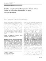
One difference between homeomorphism and homotopy is that homeomorphic spaces have same dimension while homotopy equivalent spaces need not
have same dimension. For example, the 2-ball shown in Figure 1.2(e) is homotopy equivalent to a single point though they are not homeomorphic. Any of



www.pdfgrip.com
1.1 Shapes

(a)

(d)

(b)

(e)

5

(c)

(f)

Figure 1.2. (a) 1-ball, (b) and (c) spaces homeomorphic to the 1-sphere, (d) and (e)
spaces homeomorphic to the 2-ball, and (f) an open 2-ball which is not homeomorphic
to the 2-ball in (e).

the end vertices of the segment in Figure 1.2(a) is a deformation retract of the
segment.
Isotopy
Homeomorphism and homotopy together bring a notion of similarity in spaces
which, in some sense, is stronger than each one of them individually. For example, consider a standard torus embedded in R3 . One can knot the torus (like
a knotted rope) which still embeds in R3 . The standard torus and the knotted
one are both homeomorphic. However, there is no continuous deformation of
one to the other while maintaining the property of embedding. The reason is

that the complement spaces of the two tori are not homotopy equivalent. This
requires the notion of isotopy.
An isotopy between two spaces T1 ⊆ Rk and T2 ⊆ Rk is a map ξ : T1 ×
[0, 1] → Rk such that ξ (T1 , 0) is the identity of T1 , ξ (T1 , 1) = T2 and for
each t ∈ [0, 1], ξ (·, t) is a homeomorphism onto its image. An ambient isotopy
between T1 and T2 is a map ξ : Rk × [0, 1] → Rk such that ξ (·, 0) is the identity
of Rk , ξ (T1 , 1) = T2 and for each t ∈ [0, 1], ξ (·, t) is a homeomorphism of Rk .


www.pdfgrip.com
1 Basics

6

Observe that ambient isotopy also implies isotopy. It is also known that two
spaces that have an isotopy between them also have an ambient isotopy between
them. So, these two notions are equivalent. We will call T1 and T2 isotopic if
they have an isotopy between them.
When we talk about reconstructing surfaces from sample points, we would
like to claim that the reconstructed surface is not only homeomorphic to the
sampled one but is also isotopic to it.

1.1.2 Manifolds
Curves and surfaces are a particular type of topological space called manifolds.
A neighborhood of a point x ∈ T is an open set that contains x. A topological
space is a k-manifold if each of its points has a neighborhood homeomorphic
to the open k-ball which in turn is homeomorphic to Rk . We will consider only
k-manifolds that are subspaces of some Euclidean space.
The plane is a 2-manifold though not compact. Another example of a 2manifold is the sphere S2 which is compact. Other compact 2-manifolds include
torus with one through-hole and double torus with two through-holes. One

can glue g tori together, called summing g tori, to form a 2-manifold with g
through-holes. The number of through-holes in a 2-manifold is called its genus.
A remarkable result in topology is that all compact 2-manifolds in R3 must be
either a sphere or a sum of g tori for some g ≥ 1.
Boundary
Surfaces in R as we know them often have boundaries. These surfaces have the
property that each point has a neighborhood homeomorphic to R2 except the
ones on the boundary. These surfaces are 2-manifolds with boundary. In general,
a k-manifold with boundary has points with neighborhood homeomorphic to
either Rk , called the interior points, or the halfspace Hk , called the boundary
points. The boundary of a manifold M, bd M, consists of all boundary points.
By this definition a manifold as defined earlier has a boundary, namely an empty
one. The interior of M consists of all interior points and is denoted Int M.
It is a nice property of manifolds that if M is a k-manifold with boundary,
bd M is a (k − 1)-manifold unless it is empty. The k-ball Bk is an example
of a k-manifold with boundary where bd Bk = Sk−1 is the (k − 1)-sphere and
its interior Int Bk is the the open k-ball. On the other hand, bd Sk = ∅ and
Int Sk = Sk . In Figure 1.2(a), the segment is a 1-ball where the boundary is a 0sphere consisting of the two endpoints. In Figure 1.2(e), the 2-ball is a manifold
with boundary and its boundary is the circle, a 1-sphere.
3


www.pdfgrip.com
1.1 Shapes

7

Orientability
A 2-manifold with or without boundary can be either orientable or nonorientable. We will only give an intuitive explanation of this notion. If one travels
along any curve on a 2-manifold starting at a point, say p, and considers the

oriented normals at each point along the curve, then one gets the same oriented
normal at p when he returns to p. All 2-manifolds in R3 are orientable. However,
2-manifolds in R3 that have boundaries may not be orientable. For example, the
Măobius strip, obtained by gluing the opposite edges of a rectangle with a twist,
is nonorientable. The 2-manifolds embedded in four and higher dimensions
may not be orientable no matter whether they have boundaries or not.

1.1.3 Complexes
Because of finite storage within a computer, a shape is often approximated with
finitely many simple pieces such as vertices, edges, triangles, and tetrahedra. It
is convenient and sometimes necessary to borrow the definitions and concepts
from combinatorial topology for this representation.
An affine combination of a set of points P = { p0 , p1 , . . . , pn } ⊂ Rk is a
n
αi pi , i αi = 1 and each αi is a real number. In
point p ∈ Rk where p = i=0
addition, if each αi is nonnegative, the point p is a convex combination. The
affine hull of P is the set of points that are an affine combination of P. The
convex hull Conv P is the set of points that are a convex combination of P. For
example, three noncollinear points in the plane have the entire R2 as the affine
hull and the triangle with the three points as vertices as the convex hull.
A set of points is affinely independent if none of them is an affine combination
of the others. A k-polytope is the convex hull of a set of points which has at
least k + 1 affinely independent points. The affine hull aff µ of a polytope µ is
the affine hull of its vertices.
A k-simplex σ is the convex hull of exactly k + 1 affinely independent points
P. Thus, a vertex is a 0-simplex, an edge is a 1-simplex, a triangle is a 2-simplex,
and a tetrahedron is a 3-simplex. A simplex σ = Conv T for a nonempty subset
T ⊆ P is called a face of σ . Conversely, σ is called a coface of σ . A face σ ⊂ σ
is proper if the vertices of σ are a proper subset of σ . In this case σ is a proper

coface of σ .
A collection K of simplices is called a simplicial complex if the following
conditions hold.
(i) σ ∈ K if σ is a face of any simplex σ ∈ K.
(ii) For any two simplices σ, σ ∈ K, σ ∩ σ is a face of both unless it is empty.


www.pdfgrip.com
1 Basics

8

(a)

(b)

Figure 1.3. (a) A simplicial complex and (b) not a simplicial complex.

The above two conditions imply that the simplices meet nicely. The simplices
in Figure 1.3(a) form a simplicial complex whereas the ones in Figure 1.3(b)
do not.
Triangulation
A triangulation of a topological space T is a simplicial complex K whose
underlying point set is T. Figure 1.1(b) shows a triangulation of a 2-manifold
with boundary.
Cell Complex
We also use a generalized version of simplicial complexes in this book. The
definition of a cell complex is exactly same as that of the simplicial complex with
simplices replaced by polytopes. A cell complex is a collection of polytopes
and their faces where any two intersecting polytopes meet in a face which is

also in the collection. A cell complex is a k-complex if the largest dimension
of any polytope in the complex is k. We also say that two elements in a cell
complex are incident if they intersect.

1.2 Feature Size and Sampling
We will mainly concentrate on smooth curves in R2 and smooth surfaces in
R3 as the sampled spaces. The notation will be used to denote this generic
sampled space throughout this book. We will defer the definition of smoothness
until Chapter 2 for curves and Chapter 3 for surfaces. It is sufficient to assume


www.pdfgrip.com
1.2 Feature Size and Sampling

(a)

9

(b)

(c)
Figure 1.4. (a) A curve in the plane, (b) a sample of it, and (c) the reconstructed curve.

that is a 1-manifold in R2 and a 2-manifold in R3 for the definitions and
results described in this chapter.
Obviously, it is not possible to extract any meaningful information about
if it is not sufficiently sampled. This means features of
should be represented with sufficiently many sample points. Figure 1.4 shows a curve
in the plane which is reconstructed from a sufficiently dense sample. But,
this brings up the question of defining features. We aim for a measure that

can tell us how complicated
is around each point x ∈ . A geometric structure called the medial axis turns out to be useful to define such a
measure.