Edmond c tomastik calculus applications and technology, 3rd edition brooks cole (2004)
Bạn đang xem bản rút gọn của tài liệu. Xem và tải ngay bản đầy đủ của tài liệu tại đây (7.93 MB, 769 trang )
www.pdfgrip.com
Calculus
Applications
and
Technology
THIRD EDITION
www.pdfgrip.com
This page intentionally left blank
www.pdfgrip.com
Calculus
Applications
and
Technology
THIRD EDITION
Edmond C. Tomastik
University of Connecticut
With Interactive Illustrations by
Hu Hohn, Massachusetts School of Art
Jean Marie McDill, California Polytechnic State University, San Luis Obispo
Agnes Rash, St. Joseph’s University
Australia • Canada • Mexico • Singapore • Spain
United Kingdom • United States
www.pdfgrip.com
Publisher: Curt Hinrichs
Development Editor: Cheryll Linthicum
Assistant Editor: Ann Day
Editorial Assistant: Katherine Brayton
Technology Project Manager: Earl Perry
Marketing Manager: Tom Ziolkowski
Marketing Assistant: Jessica Bothwell
Advertising Project Manager: Nathaniel Bergson-Michelson
Senior Project Manager, Editorial Production: Janet Hill
Print/Media Buyer: Barbara Britton
Production Service: Hearthside Publication
Services/Anne Seitz
Text Designer: John Edeen
Art Editor: Ann Seitz
Photo Researcher: Gretchen Miller
Copy Editor: Barbara Willette
Illustrator: Hearthside Publishing Services/Jade Myers
Cover Designer: Ron Stanton
Cover Image: Gary Holscher
Interior Printer: Quebecor/Taunton
Cover Printer: Phoenix Color Corp
Compositor: Techsetters, Inc.
COPYRIGHT © 2005 Brooks/Cole, a division of Thomson
Learning, Inc. Thomson LearningTM is a trademark used herein
under license.
Thomson Brooks/Cole
10 Davis Drive
Belmont, CA 94002
USA
ALL RIGHTS RESERVED. No part of this work covered by
the copyright hereon may be reproduced or used in any form
or by any means—graphic, electronic, or mechanical,
including but not limited to photocopying, recording, taping,
Web distribution, information networks, or information storage
and retrieval systems—without the written permission of the
publisher.
Printed in the United States of America
1 2 3 4 5 6 7 08 07 06 05 04
For more information about our products, contact us at:
Thomson Learning Academic Resource Center
1-800-423-0563
For permission to use material from this text or product,
submit a request online at
.
Any additional questions about permissions can be
submitted by email to
COPYRIGHT 2005 Thomson Learning, Inc. All Rights
Reserved. Thomson Learning WebTutorTM is a trademark
of Thomson Learning, Inc.
Library of Congress Control Number: 2004104623
Student Edition: ISBN 0-534-46496-3
Instructor’s Edition: ISBN 0-534-46498-X
Asia
Thomson Learning
5 Shenton Way #01-01
UIC Building
Singapore 068808
Australia/New Zealand
Thomson Learning
102 Dodds Street
Southbank, Victoria 3006
Australia
Canada
Nelson
1120 Birchmount Road
Toronto, Ontario M1K 5G4
Canada
Europe/Middle East/Africa
Thomson Learning
High Holborn House
50/51 Bedford Row
London WC1R 4LR
United Kingdom
Latin America
Thomson Learning
Seneca, 53
Colonia Polanco
11560 Mexico D.F.
Mexico
Spain/Portugal
Paraninfo
Calle Magallanes, 25
28015 Madrid, Spain
www.pdfgrip.com
An Overview of Third
Edition Changes
1. In this new edition we have followed a general philosophy of dividing the material
into smaller, more manageable sections. This has resulted in an increase in the
number of sections. We think this makes it easier for the instructor and the
student, gives more flexibility, and creates a better flow of material.
2. To add to the flexibility, many sections now have enrichment subsections. Material in such enrichment subsections is not needed in the subsequent text (except
possibly in later enrichment subsections). Now instructors can easily tailor the
material in the text to teach a course at different levels.
3. The third edition has even more referenced real-life examples. It is important to
realize that the mathematical models presented in these referenced examples are
models created by the experts in their fields and published in refereed journals. So
not only is the data in these referenced examples real data, but the mathematical
models based on this real data have been created by experts in their fields (and
not by us).
4. Mathematical modeling is stressed in this edition. Mathematical modeling is an
attempt to describe some part of the real world in mathematical terms. Already
at the beginning of Section 1.2 we describe the three steps in mathematical modeling: formulation, mathematical manipulation, and evaluation. We return to
this theme often. For example, in Section 5.6 on optimization and modeling we
give a six-step procedure for mathematical modeling specifically useful in optimization. Essentially every section has examples and exercises in mathematical
modeling.
5. This edition also includes many more opportunities to model by curve fitting.
In this kind of modeling we have a set of data connecting two variables, x and
y, and graphed in the xy-plane. We then try to find a function y = f (x) whose
graph comes as close as possible to the data. This material is found in a new
Chapter 2 and can be skipped without any loss of continuity in the remainder of
the text. Curve-fitting exercises are clearly marked as such.
6. The text is now technology independent. Graphing calculators or computers
work just as well with the text.
7. A disk with interactive illustrations is now included with each text. These interactive illustrations provide the student and instructor with wonderful demonstrations of many of the important ideas in the calculus. They appear in every
chapter. These demonstrations and explorations are highlighted in the text at
appropriate times. They provide an extraordinary means of obtaining deep and
clear insights into the important concepts. We are extremely excited to present
these in this format.
v
www.pdfgrip.com
vi
An Overview of Third Edition Changes
Chapter 1. Functions. This chapter now contains five sections: 1.1, Functions;
1.2, Mathematical Models; 1.3, Exponential Models; 1.4, Combinations of Functions;
and 1.5, Logarithms. The material that covered modeling with least squares has all
been moved to a new Chapter 2. Most of the material in the sections on quadratics and
special functions has been moved to the Review Appendix. A geometric definition
of continuity now appears in the first section.
Chapter 2. Modeling with Least Squares. This is a new chapter and places all
the material on least squares that was originally in Chapter 1 into this new chapter.
Instructors who wish can ignore the material in this chapter.
Chapter 3. Limits and the Derivative. This chapter has been substantially
revised. The material on the limit definition of continuity is now an “enrichment”
subsection of the first section on limits and is not needed in the remainder of the text.
The material on limits at infinity has been moved to a later chapter. The section on rates
of change now has more examples of average rates of change. More emphasis is put
on interpretations of rates of change and on units. The old section on derivatives has
been made into two sections, the first on derivatives and the second on local linearity.
The new section on derivatives has more emphasis on graphing the derivative given
the function and also on interpretations. The section on local linearity now includes
marginal analysis and the economic interpretation of the derivatives of cost, revenue,
and profits. This latter material was formerly in a later chapter.
Chapter 4. Rules for Derivatives. This chapter now includes more “intuitive,”
that is, geometrical and numerical, sketches of a number of proofs, the formal proofs
being given in enrichment subsections. Thus, a geometrical sketch of the proof for the
derivative of a constant times a function is given, and numerical evidence for the proof
for the derivative of the sum of two functions is given. The formal proofs of these,
together with the proof of the derivative of the product, are in optional subsections.
More geometrical insight has been added to the chain rule, and more emphasis is
put on determining units. The more difficult proofs in the exponential and logarithm
section have been placed in an enrichment subsection. Elasticity of demand now has
it’s own section. The introductory material on elasticity has been rewritten to make
the topic more transparent. The last section on applications on renewable resources
has been updated with timely new material.
Chapter 5. Curve Sketching and Optimization. This chapter has been extensively reorganized. The second section on the second derivative now contains only
material specific to concavity and the second derivative test and is much shorter and
much more manageable. The material on additional curve sketching that was previously in this section has been given its own section, Section 5.4. Limits at infinity are
now discussed in Section 3, having been moved from an earlier chapter. It is in this
chapter that this material is actually used, so it seems appropriate that it be located
here. The old section on optimization has been split into two sections, the first on
absolute extrema and the second on optimization and mathematical modeling. A new
section on the logistic curve has been created from material found scattered in various
sections. With its own section, new material has been added to give this important
model its proper due (although instructors can omit this material without effecting
the flow of the text).
Chapter 6. Integration. The section on substitution has been refocused to have
a more intuitive as opposed to formal approach and is now more easily accessible.
To the third section, on distance traveled, more examples of Riemann sums have
been added, and taking the limit as n → ∞ is postponed until the next section. The
section on the definite integral now contains some properties of integrals that were
not found in the last edition. The section on the fundamental theorem of calculus has
www.pdfgrip.com
An Overview of Third Edition Changes
vii
been extensively rewritten, with a different proof of the fundamental theorem given.
x
We first show that the derivative of
f (t) dt is f (x) using a geometric argument
a
using the new properties of integrals that were included in the previous section and
b
f (t) dt = F (b) − F (a), where F is an antiderivative. The
then proceed to prove
a
more formal proof is given in an enrichment subsection. Finally, a new Section 6.7
has been created to include the various applications of the integral that had been
scattered in previous sections.
Chapter 7. Additional Topics in Integration. The interactive illustrations in
the numerical integration section yield considerable insight into the subject. Students
can move from one method to another and choose any n and see the graphs and the
numerical answers immediately.
Chapter 8. Functions of Several Variables. Graphing in several variables
and visualizing the geometric interpretation of partial derivatives is always difficult.
There are several interactive illustrations in this chapter that are extremely helpful in
this regard.
Chapter 9. The Trigonometric Functions. This chapter covers an introduction
to the trigonometric functions, including differentiation and integration.
Chapter 10. Taylor Polynomials and Infinite Series. This chapter covers
Taylor polynomials and infinite series. Sections 10.1, 10.2, and 10.7 constitute a
subchapter on Taylor polynomials. Section 10.7 is written so that the reader can go
from Section 10.2 directly to Section 10.7.
Chapter 11. Probability and Calculus. This chapter is on probability. Section
11.1 is a brief review of discrete probability. Section 11.2 considers continuous probability density functions and Section 11.3 presents the expected value and variance
of these functions. Section 11.4 covers the normal distribution.
Chapter 12. Differential Equations. This chapter is a brief introduction to
differential equations and includes the technique of separation of variables, approximate solutions using Euler’s method, some qualitative analysis, and mathematical
problems involving the harvesting of a renewable natural resource.
www.pdfgrip.com
This page intentionally left blank
www.pdfgrip.com
Preface
Calculus: Applications and Technology is designed to be used in a one- or twosemester calculus course aimed at students majoring in business, management, economics, or the life or social sciences. The text is written for a student with two years
of high school algebra. A wide range of topics is included, giving the instructor
considerable flexibility in designing a course.
Since the text uses technology as a major tool, the reader is required to use a
computer or a graphing calculator. The Student’s Suite CD with the text, gives all
the details, in user friendly terms, needed to use the technology in conjunction with
the text. This text, together with the accompanying Student’s Suite CD, constitutes a
completely organized, self-contained, user-friendly set of material, even for students
without any knowledge of computers or graphing calculators.
Philosophy
The writing of this text has been guided by four basic principles, all of which are
consistent with the call by national mathematics organizations for reform in calculus
teaching and learning.
1. The Rule of Four: Where appropriate, every topic should be presented graphically, numerically, algebraically, and verbally.
2. Technology: Incorporate technology into the calculus instruction.
3. The Way of Archimedes: Formal definitions and procedures should evolve
from the investigation of practical problems.
4. Teaching Method: Teach calculus using the investigative, exploratory approach.
The Rule of Four. By always bringing graphical and numerical, as well as algebraic, viewpoints to bear on each topic, the text presents a conceptual understanding
of the calculus that is deep and useful in accommodating diverse applications. Sometimes a problem is done algebraically, then supported numerically and/or graphically
(with a grapher). Sometimes a problem is done numerically and/or graphically (with
a grapher), then confirmed algebraically. Other times a problem is done numerically
or graphically because the algebra is too time-consuming or impossible.
Technology. Technology permits more time to be spent on concepts, problem
solving, and applications. The technology is used to assist the student to think about
ix
www.pdfgrip.com
x
Preface
the geometric and numerical meaning of the calculus, without undermining the algebraic aspects. In this process, a balanced approach is presented. I point out clearly
that the computer or graphing calculator might not give the whole story, motivating
the need to learn the calculus. On the other hand, I also stress common situations
in which exact solutions are impossible, requiring an approximation technique using
the technology. Thus, I stress that the graphers are just another needed tool, along
with the calculus, if we are to solve a variety of problems in the applications.
Applications and the Way of Archimedes. The text is written for users of
mathematics. Thus, applications play a central role and are woven into the development of the material. Practical problems are always investigated first, then used to
motivate, to maintain interest, and to use as a basis for developing definitions and
procedures. Here too, technology plays a natural role, allowing the forbidding and
time-consuming difficulties associated with real applications to be overcome.
The Investigative, Exploratory Approach. The text also emphasizes an investigative and exploratory approach to teaching. Whenever practical, the text gives
students the opportunity to explore and discover for themselves the basic calculus
concepts. Again, technology plays an important role. For example, using their graphers, students discover for themselves the derivatives of x 2 , x 3 , and x 4 and then
generalize to x n . They also discover the derivatives of ln x and ex . None of this is
realistically possible without technology.
Student response in the classroom has been exciting. My students enjoy using
their computers or graphing calculators and feel engaged and part of the learning
process. I find students much more receptive to answering questions about their
observations and more ready to ask questions.
A particularly effective technique is to take 15 or 20 minutes of class time and
have students work in small groups to do an exploration or make a discovery. By
walking around the classroom and talking with each group, the instructor can elicit
lively discussions, even from students who do not normally speak. After such a
minilab the whole class is ready to discuss the insights that were gained.
Fully in sync with current goals in teaching and learning mathematics, every section in the text includes a more challenging exercise set that encourages exploration,
investigation, critical thinking, writing, and verbalization.
Interactive Illustrations. The Student’s Suite CD with interactive illustrations
is now included with each text. These interactive illustrations provide the student
and instructor with wonderful demonstrations of many of the important ideas in
the calculus. These demonstrations and explorations are highlighted in the text at
appropriate times. They provide an extraordinary means of obtaining deep and clear
insights into the important concepts. We are extremely excited to present these in
this format. They are one more important example of the use of technology and fit
perfectly into the investigative and exploratory approach.
Content Overview
Chapter 1. Section 1.0 contains some examples that clearly indicate instances when
the technology fails to tell the whole story and therefore motivates the need to learn
the calculus. This failure of the technology to give adequate information is complemented elsewhere by examples in which our current mathematical knowledge is
inadequate to find the exact values of critical points, requiring us to use some approximation technique on our computers or graphing calculators. This theme of needing
both mathematical analysis and technology to solve important problems continues
www.pdfgrip.com
Preface
xi
throughout the text. Section 1.1 begins with functions; the second section contains
applications of linear and nonlinear functions in business and economics, including
an introduction to the theory of the firm. Next is a section on exponential functions,
followed by the algebra of functions, and finally logarithmic functions.
Chapter 2. This chapter consists entirely of fitting curves to data using least
squares. It includes linear, quadratic, cubic, quartic, power, exponential, logarithmic,
and logistic regression.
Chapter 3. Chapter 3 begins the study of calculus. Section 3.1 introduces limits
intuitively, lending support with many geometric and numerical examples. Section
3.2 covers average and instantaneous rates of change. Section 3.3 is on the derivative.
In this section, technology is used to find the derivative of f (x) = ln x. From the
f (x + h) − f (x)
limit definition of derivative we know that for h small, f (x) ≈
.
h
ln(x + 0.001) − ln x
We then take h = 0.001 and graph the function g(x) =
. We see
0.001
on our grapher that g(x) ≈ 1/x. Since f (x) ≈ g(x), we then have strong evidence
that f (x) = 1/x. This is confirmed algebraically in Chapter 4. Section 3.4 covers
local linearity and introduces marginal analysis.
Chapter 4. Section 4.1 begins the chapter with some rules for derivatives. In this
section we also discover the derivatives of a number of functions using technology.
Just as we found the derivative of ln x in the preceding chapter, we graph g(x) =
f (x + 0.001) − f (x)
for the functions f (x) = x 2 , x 3 , and x 4 and then discover
0.001
from our graphers what particular function g(x) is in each case. Since f (x) ≈ g(x),
we then discover f (x). We then generalize to x n . In the same way we find the
derivative of f (x) = ex . This is an exciting and innovative way for students to find
these derivatives. Now that the derivatives of ln x and ex are known, these functions
can be used in conjunction with the product and quotient rules found in Section
4.2, making this material more interesting and compelling. Section 4.3 covers the
chain rule, and Section 4.4 derives the derivatives of the exponential and logarithmic
functions in the standard fashion. Section 4.5 is on elasticity of demand, and Section
4.6 is on the management of renewable natural resources.
Chapter 5. Graphing and curve sketching are begun in this chapter. Section
5.1 describes the importance of the first derivative in graphing. We show clearly
that the technology can fail to give a complete picture of the graph of a function,
demonstrating the need for the calculus. We also consider examples in which the
exact values of the critical points cannot be determined and thus need to resort to using
an approximation technique on our computers or graphing calculators. Section 5.2
presents the second derivative, its connection with concavity, and its use in graphing.
Section 5.3 covers limits at infinity, Section 5.4 covers additional curve sketching, and
Section 5.5 covers absolute extrema. Section 5.6 includes optimization and modeling.
Section 5.7 covers the logistic model. Section 5.8 covers implicit differentiation and
related rates. Extensive applications are given, including Laffer curves used in tax
policy, population growth, radioactive decay, and the logistic equation with derived
estimates of the limiting human population of the earth.
Chapter 6. Sections 6.1 and 6.2 present antiderivatives and substitution, respectively. Section 6.3 lays the groundwork for the definite integral by considering leftand right-hand Riemann sums. Here again technology plays a vital role. Students
can easily graph the rectangles associated with these Riemann sums and see graphically and numerically what happens as n → ∞. Sections 6.4, 6.5, and 6.6 cover the
definite integral, the fundamental theorem of calculus, and area between two curves,
www.pdfgrip.com
xii
Preface
respectively. Section 6.7 presents a number of additional applications of the integral, including average value, density, consumer’s and producer’s surplus, Lorentz’s
curves, and money flow.
Chapter 7. This chapter contains material on integration by parts, integration
using tables, numerical integration, and improper integrals.
Chapter 8. Section 8.1 presents an introduction to functions of several variables, including cost and revenue curves, Cobb-Douglas production functions, and
level curves. Section 8.2 then introduces partial derivatives with applications that
include competitive and complementary demand relations. Section 8.3 gives the
second derivative test for functions of several variables and applied application on
optimization. Section 8.4 is on Lagrange multipliers and carefully avoids algebraic
complications. The tangent plane approximations is presented in Section 8.5. Section 8.6, on double integrals, covers double integrals over general domains, Riemann
sums, and applications to average value and density. A program is given for the
graphing calculator to compute Riemann sums over rectangular regions.
Chapter 9. This chapter covers an introduction to the trigonometric functions.
Section 9.1 starts with angles, and Sections 9.2, 9.3, and 9.4 cover the sine and cosine
functions, including differentiation and integration. Section 9.5 covers the remaining
trigonometric functions. Notice that these sections include extensive business applications, including models by Samuelson and Phillips. Notice in Section 9.3 that the
derivatives of sin x and cos x are found by using technology and that technology is
used throughout this chapter.
Chapter 10. This chapter covers Taylor polynomials and infinite series. Sections 10.1, 10.2, and 10.7 constitute a subchapter on Taylor polynomials. Section 10.7
is written so that the reader can go from Section 10.2 directly to Section 10.7. Section
10.1 introduces Taylor polynomials, and Section 10.2 considers the errors in Taylor
polynomial approximation. The graphers are used extensively to compare the Taylor
polynomial with the approximated function. Section 10.7 looks at Taylor series, in
which the interval of convergence is found analytically in the simpler cases while
graphing experiments cover the more difficult cases. Section 10.3 introduces infinite
sequences, and Sections 10.4, 10.5, and 10.6 are on infinite series and includes a
variety of test for convergence and divergence.
Chapter 11. This chapter is on probability. Section 11.1 is a brief review of
discrete probability. Section 11.2 then considers continuous probability density functions, and Section 11.3 presents the expected value and variance of these functions.
Section 11.4 covers the normal distribution, arguably the most important probability
density function.
Chapter 12. This chapter is a brief introduction to differential equations and
includes the technique of separation of variables, approximate solutions using Euler’s method, some qualitative analysis, and mathematical problems involving the
harvesting of a renewable natural resource. The graphing calculator is used to graph
approximate solutions and to do some experimentation.
Important Features
Style. The text is designed to implement the philosophy stated earlier. Every chapter and section opens by posing an interesting and relevant applied problem using
familiar vocabulary; this problem is solved later in the chapter or section after the
appropriate mathematics has been developed. Concepts are always introduced intuitively, evolve gradually from the investigation of practical problems or particular
www.pdfgrip.com
Preface
xiii
cases, and culminate in a definition or result. Students are given the opportunity to
investigate and discover concepts for themselves by using the technology, including the interactive illustrations, or by doing the explorations. Topics are presented
graphically, numerically, and algebraically to give the reader a deep and conceptual
understanding. Scattered throughout the text are historical and anecdotal comments.
The historical comments not only are interesting in themselves, but also indicate that
mathematics is a continually developing subject. The anecdotal comments relate the
material to contemporary real-life situations.
Applications. The text includes many meaningful applications drawn from a
variety of fields, including over 500 referenced examples extracted from current
journals. Applications are given for all the mathematics that is presented and are used
to motivate the students. See the Applications Index.
Explorations. These explorations are designed to make the student an active
partner in the learning process. Some of these explorations can be done in class,
and some can be done outside class as group or individual projects. Not all of these
explorations use technology; some ask students to solve a problem or make a discovery
using pencil and paper.
Interactive Illustrations. The interactive illustrations provide the student and
instructor with wonderful demonstrations of many of the important ideas in the calculus. These demonstrations and explorations are highlighted in the text at appropriate
times. They provide an extraordinary means of obtaining deep and clear insights
into the important concepts. They are one more important example of the use of
technology and fit perfectly into the investigative and exploratory approach.
Worked Examples. Over 400 worked examples, including warm up examples
mentioned below, have been carefully selected to take the reader progressively from
the simplest idea to the most complex. All the steps that are needed for the complete
solutions are included.
Connections. These are short articles about current events that connect with the
material being presented. This makes the material more relevant and interesting.
Screens. About 100 computer or graphing calculator screens are shown in the
text. In almost all cases, they represent opportunities for the instructor to have the
students reproduce these on their graphers at the point in the lecture when they are
needed. This makes the student an active partner in the learning process, emphasizes
the point being made, and makes the classroom more exciting.
Enrichment Subsections. Many sections in the text have an enrichment subsection at the end. Sometimes this subsection will include proofs that not all instructors
might wish to present. Sometimes this subsection will include material that goes
beyond what every instructor might wish to cover for the particular topic. It seems
likely that most instructors will use some of the enrichment subsections, but very few
will use all of them. This feature gives added flexibility to the text.
Warm Up Exercises. Immediately preceding each exercise set is a set of warm
up exercises. These exercises have been very carefully selected to bridge the gap
between the exposition in the section and the regular exercise set. By doing these
exercises and checking the complete solutions provided, students will be able to test
or check their comprehension of the material. This, in turn, will better prepare them
to do the exercises in the regular exercise set.
Exercises. The book contains over 2600 exercises. The exercises in each set
gradually increase in difficulty, concluding with the more challenging exercises mentioned below. The exercise sets also include an extensive array of realistic applications from diverse disciplines, including numerous referenced examples extracted
from current journals.
www.pdfgrip.com
xiv
Preface
More Challenging Exercises. Every section in the text includes a more challenging exercise set that encourages exploration, investigation, critical thinking, writing,
and verbalization.
Mathematical Modeling Exercises. Every section in the text has exercises
that provide the opportunity for mathematical modeling. The discipline of taking
a problem and translating it into a mathematical equation or construct may well be
more important than learning the actual material.
Modeling Exercises by Curve Fitting. Some instructors are interested in curve
fitting using least squares. Ample exercises are provided throughout the text that use
curve fitting as part of the problem.
End-of-Chapter Cases. These cases, found at the end of each chapter, are
especially good for group assignments. They are interesting and will serve to motivate
the mathematics student.
Learning Aids.
• Boldface is used when new terms are defined.
• Boxes are used to highlight definitions, theorems, results, and procedures.
• Remarks are used to draw attention to important points that might otherwise be
overlooked.
• Warnings alert students against making common mistakes.
• Titles for worked examples help to identify the subject.
• Chapter summary outlines at the end of each chapter conveniently summarize
all the definitions, theorems, and procedures in one place.
• Review exercises are found at the end of each chapter.
• Answers to selected exercises and to all the review exercises are provided in an
appendix.
Instructor Aids
• The Instructor’s Suite CD contains electronic versions of the Instructor’s Solutions Manual, Test Bank, and a Microsoftđ Power-Pointđ presentation tool.
ã The Instructors Solutions Manual provides completely worked solutions to
all the exercises and to all the Explorations.
• The Student Solutions Manual contains the completely worked solutions to
selected exercises and to all chapter review exercises. Between the two manuals
all exercises are covered.
• The Graphing Calculator Manual and Microsoft® Excel Manual, available electronically, have all the details, in user friendly terms, on how to carry out any
of the graphing calculator operations and Excel operations used in the text. The
Graphing Calculator Manual includes the standard calculators and computer algebra systems.
• The Test Bank written by James Ball (University of Indiana) includes a combination of multiple-choice and free-response test questions organized by section.
• A BCA/iLrn Instructor Version allows instructors to quickly create, edit, and
print tests or different versions of tests from the set of test questions accompanying
the text. It is available in IBM or Mac versions.
www.pdfgrip.com
Preface
xv
Custom Publishing. Courses in business calculus are structured in various
ways, differing in length, content, and organization. To cater to these differences,
Brooks/Cole Publishing is offering Applied Calculus with Technology and Applications in a custom-publishing format. Instructors can rearrange, add, or cut chapters
to produce a text that best meets their needs. Chapters on differential equations,
trigonometric functions, Taylor polynomials and infinite series, and probability are
also available.
Thomson Brooks/Cole is working hard to provide the highest-quality service and
product for your courses. If you have any questions about custom publishing, please
contact your local Brooks/Cole sales representatives.
Acknowledgments. I owe a considerable debt of gratitude to Curt Hinrichs,
Publisher, for his support in initiating this project, for his insightful suggestions in
preparing the manuscript, and for obtaining the services of several people, mentioned
below, who created the interactive illustrations that are in this text. These interactive
illustrations are wonderful enhancements to the text.
I wish to thank Hu Hohn, Jean Marie McDill, and Agnes Rash for their considerable work and creativity in developing all of the Interactive Illustrations that are in
this text.
I wish also to thank the other editorial, production, and marketing staff of
Brooks/Cole: Katherine Brayton, Ann Day, Janet Hill, Hal Humphrey, Cheryll
Linthicum, Earl Perry, Jessica Perry, Barbara Willette, Joseph Rogove, and Marlene Veach. I wish to thank David Gross and Julie Killingbeck for doing an excellent
job ensuring the accuracy and readability of this edition.
I would like to thank Anne Seitz for an outstanding job as Production Editor and
to thank Jade Myers for the art and Barbara Willette for the copyediting.
I would like to thank the Mathematics Department at the University of Connecticut for their collective support, with particular thanks to Professors Jeffrey Tollefson,
Charles Vinsonhaler, and Vince Giambalvo, and to our computer manager Kevin
Marinelli.
I would especially like to thank my wife Nancy Nicholas Tomastik, since without
her support, this project would not have been possible.
Many thanks to all the reviewers listed below.
Bruce Atkinson, Samford University; Robert D. Brown, University of Kansas;
Thomas R. Caplinger, University of Memphis; Janice Epstein, Texas A&M University; Tim Hagopian, Worcester State College. Fred Hoffman, Florida Atlantic
University; Miles Hubbard, Saint Cloud State University; Kevin Iga, Pepperdine
University; David L. Parker, Salisbury University; Georgia Pyrros, University of
Delaware; Geetha Ramanchandra, California State University, Sacramento; Jennifer
Stevens, University of Tennessee; Robin G. Symonds, Indiana University, Kokomo;
Stuart Thomas, University of Oregon at Eugene; Jennifer Whitfield, Texas A&M
University; and Richard Witt, University of Wisconsin, Eau Claire.
www.pdfgrip.com
This page intentionally left blank
www.pdfgrip.com
Table of Contents
1
Functions
1.0
1.1
1.2
1.3
1.4
1.5
2
Introduction to Calculus
Limits
142
Rates of Change
160
The Derivative
188
Local Linearity
205
138
139
Rules for the Derivative
4.1
4.2
4.3
4.4
4.5
4.6
100
Method of Least Squares
100
Quadratic Regression
112
Cubic, Quartic, and Power Regression
118
Exponential and Logarithmic Regression
123
Logistic Regression
127
Selecting the Best Model
131
Limits and the Derivative
3.0
3.1
3.2
3.3
3.4
4
Graphers Versus Calculus
4
Functions
5
Mathematical Models
24
Exponential Models
50
Combinations of Functions
70
Logarithms
78
Modeling with Least Squares
2.1
2.2
2.3
2.4
2.5
2.6
3
2
222
Derivatives of Powers, Exponents, and Sums
223
Derivatives of Products and Quotients
244
The Chain Rule
254
Derivatives of Exponential and Logarithmic Functions
Elasticity of Demand
275
Management of Renewable Natural Resources
284
264
xvii
www.pdfgrip.com
xviii
Table of Contents
5
Curve Sketching and Optimization
5.1
5.2
5.3
5.4
5.5
5.6
5.7
5.8
6
Integration
6.1
6.2
6.3
6.4
6.5
6.6
6.7
7
380
396
Antiderivatives
398
Substitution
408
Estimating Distance Traveled
416
The Definite Integral
432
The Fundamental Theorem of Calculus
Area Between Two Curves
461
Additional Applications of the Integral
447
473
Additional Topics in Integration
7.1
7.2
7.3
7.4
8
The First Derivative
295
The Second Derivative
314
Limits at Infinity
330
Additional Curve Sketching
342
Absolute Extrema
350
Optimization and Modeling
360
The Logistic Model
370
Implicit Differentiation and Related Rates
488
Integration by Parts
488
Integration Using Tables
495
Numerical Integration
500
Improper Integrals
512
Functions of Several Variables
8.1
8.2
8.3
8.4
8.5
8.6
294
Functions of Several Variables
523
Partial Derivatives
538
Extrema of Functions of Two Variables
Lagrange Multipliers
564
Tangent Plane Approximations
572
Double Integrals
578
522
552
Chapters 9–12 are included on the Students’ Suite CD with this book.
9
The Trigonometric Functions
9.1
9.2
9.3
9.4
9.5
Angles
9.2
The Sine and the Cosine
9.15
Differentiation of the Sine and Cosine Functions
Integrals of the Sine and Cosine Functions
9.48
Other Trigonometric Functions
9.54
9.38
www.pdfgrip.com
Table of Contents
10
Taylor Polynomials and Infinite Series
10.1
10.2
10.3
10.4
10.5
10.6
10.7
11
Probability and Calculus
11.1
11.2
11.3
11.4
12
11.24
Differential Equations
12.2
Separation of Variables
12.11
Approximate Solutions to Differential Equations
Qualitative Analysis
12.35
Harvesting a Renewable Resource
12.46
Review
A.1
A.2
A.3
A.4
A.5
A.6
A.7
A.8
B
Discrete Probability
11.2
Continuous Probability Density Functions
Expected Value and Variance
11.37
The Normal Distribution
11.50
Differential Equations
12.1
12.2
12.3
12.4
12.5
A
Taylor Polynomials
10.2
Errors in Taylor Polynomial Approximation
10.18
Infinite Sequences
10.28
Infinite Series
10.38
The Integral and Comparison Tests
10.53
The Ratio Test and Absolute Convergence
10.64
Taylor Series
10.73
B.1
B.2
598
Exponents and Roots
598
Polynomials and Rational Expressions
603
Equations
608
Inequalities
613
The Cartesian Coordinate System
618
Lines
626
Quadratic Functions
640
Some Special Functions and Graphing Techniques
Tables
662
Basic Geometric Formulas
Tables of Integrals
665
662
Answers to Selected Exercises
Index
12.24
I-1
AN-1
651
xix
www.pdfgrip.com
1
Functions
1.0 Graphers Versus Calculus
1.1 Functions
1.2 Mathematical Models
1.3 Exponential Models
1.4 Combinations of Functions
1.5 Logarithms
This chapter covers functions, which form the basis of calculus. We
introduce the notion of a function, introduce a variety of functions, and
then explore the properties and graphs of these functions.
CASE STUDY
We consider here certain data found in a recent detailed
study by Cotterill and Haller1 of the costs and pricing
for a number of brands of breakfast cereals. The data
shown in Table 1.1 were in support of Cotterill’s testimony as an expert economic witness for the state of
New York in State of New York v. Kraft General Foods
et al. It is the first, and probably only, full-scale attempt to present in a federal district court analysis of
a merger’s impact using scanner-generated brand-level
data and econometric techniques to estimate brand- and
category-level responses of demand to pricing. Keep
in mind that the data in this study were obtained from
Kraft by court order as part of New York’s challenge
of the acquisition of Nabisco Shredded Wheat by Kraft
General Foods. Otherwise, such data would be extremely difficult, and most likely impossible, to obtain.
1
2
Ronald W. Cotterill and Lawrence E. Haller. 1997. An economic
analysis of the demand for RTE cereal: product market definition and unilateral market power effects. Research Report No. 35.
Food Marketing Policy Center. University of Connecticut.
Table 1.1
Item
Manufacturing cost:
Grain
Other ingredients
Packaging
Labor
Plant costs
Total manufacturing costs
Marketing expenses:
Advertising
Consumer promo
(mfr. coupons)
Trade promo (retail in-store)
Total marketing costs
Total costs per unit
$/lb
$/ton
0.16
0.20
0.28
0.15
0.23
1.02
320
400
560
300
460
2040
0.31
620
0.35
0.24
0.90
1.92
700
480
1800
3840
www.pdfgrip.com
The manufacturer obtains a price of $2.40 a pound, or
$4800 a ton. Nevo2 estimated the costs of construction
of a typical plant to be $300 million. We want to find
the cost, revenue and profit equations.
Let x be the number of tons of cereal manufactured
and sold, and let p be the price of a ton sold. Notice
that, according to Table 1.1, the cost to manufacture
each ton of cereal is $3840. So the cost of manufacturing x tons is 3840x dollars. To obtain (total) cost, we
need to add to this the cost of the plant itself, which was
$300 million. To simplify the cost equation, let total
cost C be given in thousands of dollars. Then the total
cost C, in thousands of dollars, for manufacturing x
tons of cereal is given by C = 300,000 + 3.84x. This
is graphed in Figure 1.1.
A ton of cereal sold for $4800. So selling x tons
of cereal returned revenue of 4800x dollars. If we let
revenue R be given in thousands of dollars, then the
revenue from selling x tons of cereal is R = 4.8x. This
is shown in Figure 1.1.
2
Aviv Nevo. 2001. Measuring market power in the ready-to-eat
cereal industry. Econometrica 69(2):307–342.
R, C, P
R = 4.8x
2,000,000
C = 300,000 + 3.84x
1,500,000
1,000,000
500,000
0
P = R−C
100,000 200,000 300,000 400,000 500,000 x
Figure 1.1
Profits are always just revenue less costs. So if P
is profits in thousands of dollars, then
P = R − C = (4.8x) − (3.840x + 300,000)
= 0.96x − 300,000
This equation is also graphed in Figure 1.1.
We might further ask how many tons of cereal we
need to manufacture and sell before we break even.
The answer can be found in Example 1 of Section 1.2
on page 28.
3
www.pdfgrip.com
4
CHAPTER 1
Functions
1.0
Graphers Versus Calculus
We (informally) call a graph complete if the portion of the graph that we see in the
viewing window suggests all the important features of the graph. For example, if
some interesting feature occurs beyond the viewing window, then the graph is not
complete. If the graph has some important wiggle that does not show in the viewing
window because the scale of the graph is too large, then again the graph is not
complete. Unfortunately, no matter how large or small the scale of the graph, we can
never be certain that some interesting behavior might not be occurring outside the
viewing window or some interesting wiggles aren’t hidden within the curve that we
see. Thus, if we use only a graphing utility on a graphing calculator or computer, we
might overlook important discoveries. This is one reason why we need to carefully
do a mathematical analysis.
If you do not know how to use your graphing calculator or computer, consult
the Technology Resource Manual that accompanies this text. Any time a term or
operation is introduced in this text, the Technology Resource Manual clearly explains
the term or operation and gives all the necessary keystrokes. Therefore, you can read
the text and the manual together.
EXAMPLE 1
Complete Graphs
Graph y = x 4 − 12x 3 + x 2 − 2 in a window with dimensions [−10, 10] by [−10, 10]
using your grapher. If this is not satisfactory, find a better window.
[–10, 10] × [–10, 10]
Screen 1.1
A graph of y = x 4 − 12x 3 +
x 2 − 2 in a standard window.
Solution
The graph is shown in Screen 1.1. You might reflect whether this is a complete graph.
Suppose, for example, that x is huge, say, a billion. Then the first term x 4 can be
written as x · x 3 , or one billion times x 3 . The second term −12x 3 can be thought of
as −12 times x 3 . Since −12 is insignificant compared to one billion, the term −12x 3
is insignificant compared to x 4 . The other terms x 2 and 10 are even less significant.
So the polynomial for huge x should be approximately equal to the leading term x 4 .
But x 4 is a huge positive number when x is huge. This is not reflected in the graph
found in Screen 1.1. Therefore, we should take a screen with larger dimensions. If we
set the dimensions of our viewing window to [−5, 14] by [−2500, 1000], we obtain
Screen 1.2. Notice the missing behavior we have now discovered.
EXAMPLE 2
Complete Graphs
4
Graph y = x − 2x 3 + x 2 + 10 using a window with dimensions [−10, 10] by
[−10, 10] on your grapher. If this is not satisfactory, find a better window.
[–5, 14] × [–2500, 1000]
Screen 1.2
A graph of y = x 4 − 12x 3 +
x 2 − 2 showing some hidden
behavior.
Solution
If we graph using the given viewing window, we see nothing! Try it. Where is the
graph? We must examine the function more carefully to see which window to use.
Notice that when x = 0, y = 10. We then might think to center our screen on the point
(0, 10). So take a screen with dimensions [−10, 10] by [0, 20] and obtain Screen 1.3.
Now we see something! But are we seeing everything? Either using the ZOOM
feature of your grapher to ZOOM about (0, 10) or setting the screen dimensions to
www.pdfgrip.com
1.1 Functions
5
[−2.5, 2.5] by [7.5, 12.5], obtain Screen 1.4. Notice the missing behavior, in the
form of a wiggle, that we have now discovered.
[–10, 10] × [0, 20]
[–2.5, 2.5] × [7.5, 12.5]
Screen 1.3
Screen 1.4
A graph of y = x 4 − 2x 3 +
x 2 + 10.
A graph of y = x 4 − 2x 3 +
x 2 + 10 showing some hidden
behavior.
The previous two examples indicate the shortfalls of using a graphing utility
on a graphing calculator or computer. Determining the dimensions of the viewing
screen can represent a major difficulty. We can never know whether some interesting
behavior is taking place just outside the viewing screen, no matter how large it is.
Also, if we use only a graphing utility, how can we ever know whether there are some
hidden wiggles somewhere in the graph? We cannot ZOOM everywhere and forever!
We will be able to determine complete graphs by expanding our knowledge of
mathematics, and, in particular, by using calculus. In Chapter 5 we will use calculus
to find all the wiggles and hidden behavior of a graph.
1.1
Functions
Definition of Function
Graphs of Functions
Increasing, Decreasing, Concavity, and Continuity
Applications and Mathematical Modeling
The Bettmann Archive/Hutton
Lejeune Dirichlet, 1805–1859
Dirichlet was one of the mathematical giants of the 19th century. He
formulated the notion of function that is still used today and is also
known for the Dirichlet series, the Dirichlet function, the Dirichlet
principle, and the Dirichlet problem. The Dirichlet problem is fundamental to the study of thermodynamics and electrodynamics. Although described as noble, sincere, humane, and possessing a modest
disposition, Dirichlet was known as a dreadful teacher. He was also a
failure as a family correspondent. When his first child was born, he
neglected to inform his father-in-law, who, when he found out about
the event, commented that Dirichlet might have at least written a note
saying “2 + 1 = 3.”
www.pdfgrip.com
6
CHAPTER 1
Functions
APPLICATION State Income Tax
The following instructions are given on the Connecticut state income tax form to
determine your income tax.
If your taxable income is less or equal to $16,000, multiply by 0.03. If it is
more that $16,000, multiply the excess over $16,000 by 0.045 and add $480.
Let x be your taxable income. Now write a formula that gives your state
income tax for any value of x. Use this formula to find your taxes if your taxable
income is $15,000 and also $20,000. See Example 12 on page 16 for the answer.
Definition of Function
Table 1.2
Country
Capital City
Afghanistan
Albania
Algeria
Angola
Argentina
Armenia
Australia
Austria
Kabul
Tirana
Algiers
Luanda
Buenos Aires
Yerevan
Canberra
Vienna
We are all familiar with the correspondence between an element in one set and an
element in another set. For example, to each house there corresponds a house number,
to each automobile there corresponds a license number, and to each individual there
corresponds a name.
Table 1.2 lists eight countries and the capital city of each. The table indicates that
to each country there corresponds a capital city. Notice that there is one and only one
capital city for each country. Table 1.3 gives the gross domestic product (GDP) for
the United States in trillions of (current) dollars for each of 12 recent years.3 Again,
there is one and only one GDP associated with each year.
Table 1.3
Year
U.S. GDP
Year
(trillions)
1990
1991
1992
1993
1994
1995
$5.8
6.0
6.3
6.6
7.1
7.4
U.S. GDP
(trillions)
1996
1997
1998
1999
2000
2001
$7.8
8.3
8.8
9.3
10.0
10.2
We call any rule that assigns or corresponds to each element in one set precisely
one element in another set a function. Thus, the correspondences indicated in Tables
1.2 and 1.3 are functions.
As we have seen, a table can represent a function. Functions can also be represented by formulas. For example, suppose you are going a steady 40 miles per hour
in a car. In one hour you will travel 40 miles; in two hours you will travel 80 miles;
and so on. The distance you travel depends on (corresponds to) the time. Indeed, the
equation relating distance (d), velocity (v), and time (t), is d = v · t. In our example,
we have d = 40 · t. We can view this as a correspondence or rule: Given the time
t in hours, the rule gives a distance d in miles according to d = 40 · t. Thus, given
t = 3, d = 40 · 3 = 120. Notice carefully how this rule is unambiguous. That is,
3
Statistical Abstract of the United States, 2002.