Geoffrey c berresford, andrew m rockett brief applied calculus, 5th edition brooks cole (2010)(1)
Bạn đang xem bản rút gọn của tài liệu. Xem và tải ngay bản đầy đủ của tài liệu tại đây (8.35 MB, 672 trang )
www.pdfgrip.com
INDEX OF APPLICATIONS
Titles or page numbers in italics indicate applications of greater generality or significance, most including source
citations that allow those interested to pursue these topics in more detail.
Athletics
Altitude and Olympic games, 272
Athletic field design, 219
Cardiovascular zone, 49
Disappearance of the .400 baseball
hitter, 543
Fastest baseball pitch, 174
Fluid absorption, 420
How fast do old men slow down?, 303
Juggling, 48
Muscle contraction, 48, 248
Olympic medals, 507, 520
Pole vaulting improvement, 295
Pythagorean baseball standings,
507, 520
World record 100-meter run, 303
World record mile run, 3, 17
Biomedical Sciences
AIDS, 151
Allometry, 30, 31, 486
Aortic volume, 364
Aspirin dose-response, 190
Bacteria, 190, 220, 248, 272, 376, 470
Blood flow, 122, 162, 175, 520
and Reynolds number, 304
Blood vessel volume, 570
Body surface area, 506
Body temperature, 137, 138, 335, 407
Cardiac output, 569
Cell growth, 48, 346, 468
Chernobyl radioactive
contamination, 272
Cholesterol reduction, 400
Contagion, 230
Coughing, 220
Drug absorption, 364, 443, 484
Drug concentration, 228, 304, 319
Drug dosage, 271, 287, 288, 302,
320, 420, 531
Drug dose-response curve, 204, 205
Drug sensitivity, 162
Efficiency of animal motion, 220, 252
Epidemics, 121, 338, 345, 363, 480,
484, 492
Fever, 150
Fever thermometers, 491, 492
Fick’s law, 471
Future life expectancy, 19
Gene frequency, 424, 430
Glucose levels, 469, 485
Gompertz growth curve, 289, 304,
443, 486
Half-life of a drug, 289
Heart function, 471
Heart medication, 191
Heart rate, 31
Height of a child, 363
Heterozygosity, 289
Leukemic cell growth, 68
Life expectancy, 19
Life expectancy and education, 124
Longevity and exercise, 218
Lung cancer and asbestos, 123
Medication ingestion, 254
Mosquitoes, 271
Murrell’s rest allowance, 139
Nutrition, 586
Oxygen consumption, 507
Penicillin dosage, 281
Poiseuille’s law and blood flow,
249, 365
Pollen count, 217
Population and individual
birthrate, 486
Reed-Frost epidemic model, 272
Ricker recruitment, 289, 304
Smoking and longevity, 543
Tainted meat, 50
Tumor growth, 248
Weight of a teenager, 401, 405
Environmental
Sciences
Air temperature and altitude, 73
Animal size, 72
Average air pollution, 582
Beverton-Holt recruitment curve,
20, 139
Biodiversity, 31
Carbon dioxide pollution, 73
Carbon monoxide pollution, 162
Consumption of natural resources,
341, 346, 347, 363, 404, 490
Cost of cleaner water, 128
Deer population, 484
Flexfast Rubber Company, 469
Global temperatures, 150, 335
Greenhouse gases and global
warming, 162, 405
Growth of an oil slick, 156
Harvest yield, 223, 228
Light penetrating seawater, 271
Maximizing farm revenue, 253
Maximum sustainable yield, 235,
237, 237, 254
Nuclear waste, 288
Pollution, 218, 335, 375, 396,
401, 420
Pollution and absenteeism, 544
Predicting animal population, 479
Radioactive medical tracers, 287
Radioactive waste, 489
Rain forest depletion, 287
Sea level, 150
Sulfur oxide pollution, 245
Tag and recapture estimates, 506
Water quality, 122, 137, 491
Water reservoir average depth, 397
Water usage, 59
Wind power, 49, 69, 218
World solar cell production, 302
Management Science,
Business, and
Economics
Advertising, 74, 107, 121, 272, 287,
320, 493, 585
Airline passenger miles, 32, 62
www.pdfgrip.com
Apple stock price, 315
Asset appreciation, 270
AT&T net income, 197, 205, 335
AT&T stock price, 347
AudioTime, 121
Average sales, 400
Balance of trade, 377, 406
Boeing Corporation, 26, 74
Book sales, 490
Bottled water, 69
Break-even point, 41, 48, 74
Capital value of an asset, 365, 442
Car phone sales, 484
Car rentals, 73
CD sales, 138
Cigarette price and demand, 321
Cobb-Douglas production
function, 506, 520
Competition and collusion,
528–530, 532
Competitive commodities, 521
Complementary commodities, 521
Compound interest, 376
Compound interest growth
times, 289
Computer expenditures, 492
Computer sales, 17
Consumer expenditure, 296,
303, 321
Consumer price index, 543
Consumers’ surplus, 381, 406
Continuous annuity, 469
Copier repair, 218
Cost, 330, 334, 356, 363, 393, 400,
404, 405, 407, 419, 431, 489
Cost function, 36, 47, 497, 506
Cumulative profit, 378
Demand equation, 242, 247
Depreciation, 319
Digital camera sales, 197, 484
Diminishing returns, 506
DVD sales, 32
Elasticity of demand, 311, 316, 317,
321, 468
Elasticity of supply, 317
Energy usage, 17
Estimating additional profit, 563
EZCie LED flashlight, 115
Gini index, 406
Gross domestic product, 307, 331
Gross world product, 454
Handheld computers, 68
Honeywell International, 108
Income tax, 67
Insurance reserves, 68
Interest compounded
continuously, 93
Investment growth, 453
Learning curve in airplane
production, 26, 31, 172
Least cost rule, 559
Lot size, 236–238, 254
Macintosh computers, 43, 101, 376
Marginal and average cost, 191
Marginal average cost, 130,
137, 173
Marginal average profit, 137, 173
Marginal average revenue, 137
Marginal cost, 115, 121, 161
Marginal productivity, 585
of capital, 514
of labor, 514
Marginal profit, 174, 175, 519
Marginal utility, 122
Marketing to young adults, 121
Maximizing present value, 321
Maximizing production, 552, 558
Maximum production, 587
Maximum profit, 41, 48, 74, 211,
218, 222, 227, 229, 253, 526,
531, 532, 585, 586
Maximum revenue, 219, 227, 303,
321, 532
MBA salaries, 17
Microsoft net income, 205, 335, 376
Mineral deposit value, 582
Minimizing inventory costs,
231, 233
Minimizing package materials, 224
Minimum cost, 253
Mobile phones, 27, 32
MP3 players, 32, 197, 484
National debt, 150, 316
Net savings, 377
Oil demand, 320
Oil prices, 227
Oil well output, 442
Optical computer mice, 173
Pareto’s law of income
distribution, 365
Pasteurization temperature, 107
Per capita cigarette production, 218
Per capita national debt, 138
Per capita personal income, 17
POD (printing on demand), 130
PowerZip, 121
Predicting sales, 534, 542
Present value of a continuous
stream of income, 415, 419,
420, 489
Present value of preferred
stock, 443
Price and quantity, 221
Price discrimination, 531, 532, 585
Producers’ surplus, 383
Product recognition, 420, 483
Product reliability, 442
Production possibilities, 558
Production runs, 237, 254
Profit, 150, 151, 195, 244, 248, 254,
377, 515, 569
Pulpwood forest value, 220
Quality control, 272
Quest Communication, 49
Research expenditures, 68
Research In Motion stock price,
315, 347
Returns to scale, 506
Revenue, 74, 108, 204, 248, 254,
334, 401, 419
Rule of .6, 30
Rule of 72, 289
Salary, 47
Sales, 137, 173, 204, 247, 248, 250,
302, 320, 345, 363, 364, 375,
443, 470, 481, 493, 520, 587
Sales from celebrity
endorsement, 369
Satellite radio, 19, 73
Simple interest, 73
Slot machines, 18
Southwest Airlines, 49
Stock “limiting” market value, 484
Straight-line depreciation, 18, 72
Super Bowl ticket costs, 545
Supply, 248, 250
Tax revenue, 226, 228
Temperature, 204
Timber forest value, 209, 218
Total productivity, 357
www.pdfgrip.com
Total profit, 404
Total sales, 340, 400, 423, 430,
483, 492
Total savings, 346
U.S. oil production, 69
Value of a building, 470
Value of an MBA, 520
Warranties, 443
Word Search Maker, 172
Work hours, 248
Personal Finance and
Management
Accumulation of wealth, 469
Annual percentage rate (APR),
267, 270
Art appreciation, 335, 473
Automobile depreciation, 302
Automobile driving costs, 542
Central Bank of Brazil bonds, 288
Cézanne painting appreciation, 271
College trust fund, 270
Comparing interest rates, 266,
271, 319
Compound interest, 162, 174, 261,
302, 319, 406
Continuous compounding, 265
Cost of maintaining a home, 346
Depreciating a car, 262, 286
Earnings and calculus, 273, 302
European Bank bonds, 288
Federal income tax, 56
Home appreciation, 483
Honus Wagner baseball card, 271
Income tax, 68
Investment growth times, 279, 280,
286, 288, 320
Loan sharks, 270
Parking space in Manhattan, 72
Personal wealth, 465, 491
Picasso painting appreciation, 286
Present value, 262, 266, 270
Price-earnings ratio, 505
Rate of return, 272
Real estate, 406
Solar water heater savings,
347, 404
Stamp appreciation, 483
Stock price, 406
Stock yield, 505
Toyota Corolla depreciation, 271
Value of an investment, 346
Zero coupon bond, 270, 271
Social and Behavioral
Sciences
Absenteeism, 532
Advertising effectiveness, 288
Age at first marriage, 18
Campaign expenses, 229
Cell phone usage, 288
Cephalic index, 506
Cigarette tax revenue, 253
Cobb-Douglas production
function, 498
Cost of congressional victory, 545
Cost of labor contract, 378
Crime, 543
Dating older women, 287
Demand for oil, 316
Diffusion of information, 284, 287,
302, 303, 320, 475
Divorces, 346
Early human ancestors, 287
Ebbinghaus model of memory, 302
Education and income, 287
Election costs, 272
Employment seekers, 431
Equal pay for equal work, 18
Forgetting, 272, 287
Fund raising, 420
GDP relative growth rate, 321
Gender pay gap, 495
Gini index of income distribution,
385, 387
Health care expenses, 75
Health club attendance, 48
“Iceman”, 288
Immigration, 50, 107
IQ, 450, 453
Learning, 107, 116, 122, 162, 190,
283, 287, 320, 335, 363, 405,
476, 484, 492
Liquor and beer: elasticity and
taxation, 316
Longevity, 49
Lorenz curve, 387
Marriages, 363
Mazes, 442
Most populous country, 271
New Jersey cigarette taxes, 317
Population relative rate of
change, 321
Practice and rest, 531
Practice time, 375
Prison terms, 442
Procrastination, 521
Repetitive tasks, 364, 400, 405
Response rate, 431
Smoking and education, 122
Smoking and income, 18
Spread of rumors, 480, 484, 492
Status, income, and education, 161,
162, 205, 520
Stevens’ Law of Psychophysics, 177
Stimulus and response, 205
Traffic accidents, 249
Violent crime, 586
Voting, 484
Welfare, 249
World energy output, 286
World population, 67, 146, 271
Topics of General
Interest
Accidents and driving speed, 124
Aging of America, 586
Aging world population, 545
Airplane flight path, 190, 205
Approximation of , 454
Area between curves, 364, 400,
420, 442
Automobile age, 490
Automobile fatalities, 485
Average population, 400, 588
Average temperature, 375, 577, 582
Birthrate in Africa, 377
Boiling point and altitude, 47
Box design, 253, 254, 506
Building design, 558
Bus shelter design, 229
Carbon 14 dating, 257, 282,
287, 288
Cave paintings, 287
Cell phones, 68
Cigarette smoking, 323, 364
College tuition, 123
www.pdfgrip.com
Consumer fraud, 270
Container design, 557, 558, 587
Cooling coffee, 272, 302
Cost of college education, 545
Dam construction, 364
Dam sediment, 484
Dead Sea Scrolls, 282
Designing a tin can, 549
Dinosaurs, 30
Does money buy happiness?, 18
Dog years, 68
Driving accidents and age, 218
Drug interception, 191
Drunk driving, 545
Duration of telephone calls, 442
Electrical consumption, 363
Emergency stopping distance, 569
Estimating error in calculating
volume, 564, 566
Eternal recognition, 409
Expanding ripples, 243
Fencing a region, 557
First-class mail, 93
Fossils, 320
Freezing of ice, 346
Friendships, 469
Fuel economy, 138, 217, 218
Fuel efficiency, 252
Fund raising, 483
Georgia population growth, 286
Grades, 17
Graphics design, 377, 406
Gravity model for telephone calls, 506
Gutter design, 219
Hailstones, 248
Happiness and temperature, 163
Highway safety, 520
Ice cream cone price increases, 363
Impact time of a projectile, 48
Impact velocity, 48, 150
Internet access, 13, 122
Internet host computers, 420
Largest enclosed area, 213, 219,
228, 252, 547
Largest postal package, 228, 557, 558
Largest product with fixed
sum, 219
Lives saved by seat belts, 378
Manhattan Island purchase, 270
Maximum height of a bullet, 150
Measurement errors, 569
Melting ice, 254
Mercedes-Benz Brabus Rocket
speed, 335
Millwright’s water wheel rule, 218
Minimizing cost of materials, 228
Minimum perimeter rectangle, 229
Moore’s law of computer
memory, 319
Most populous states, 268, 272
Newsletters, 49
Nuclear meltdown, 271
“Nutcracker man”, 320
Oldest dinosaur, 288
Package design, 214, 219, 220,
253, 558
Page layout, 229
Parking lot design, 219
Permanent endowments, 437, 441,
444, 490
Population, 107, 162, 174, 316, 364,
404, 420, 430, 486, 489
Porsche Cabriolet speed, 334
Postage stamps, 492, 545
Potassium 40 dating, 287, 288
Raindrops, 485
Rate of growth of a circle, 172
Rate of growth of a sphere, 173
Relative error in calculations,
569, 587
Relativity, 93
Repetitive tasks, 363
Richter scale, 31
Rocket tracking, 249
Scuba dive duration, 506, 569
Seat belt use, 19
Shroud of Turin, 257, 287
Smoking, 543
Smoking and education, 49
Smoking mortality rates, 536
Snowballs, 248
Soda can design, 253
Speed and skid marks, 32
Speeding, 249
St. Louis Gateway Arch, 273
Stopping distance, 47
Superconductivity, 77, 93
Survival rate, 175
Suspension bridge, 454
Telephone calls, 569
Temperature conversion, 17
Thermos bottle temperature, 320
Time of a murder, 469
Time saved by speeding, 131
Total population of a region, 582
Total real estate value, 588
Traffic safety, 122
Tsunamis, 48
Typing speed, 283
U.S. population, 406
Unicorns, 253
United States population, 367, 375
Velocity, 149–151, 174
Velocity and acceleration, 144
Volume and area of a divided
box, 500
Volume of a building, 582
Volume under a tent, 576
Warming beer, 303
Water pressure, 47
Waterfalls, 31
Wheat yield, 543
Wind speed, 71
Windchill index, 150, 498, 507,
520, 569
Window design, 219
Wine appreciation, 228
World oil consumption, 453
World population, 302, 539
World’s largest city: now and
later, 319
Young-adult population, 335
www.pdfgrip.com
This page intentionally left blank
www.pdfgrip.com
Brief Applied
Calculus
FIFTH EDITION
Geoffrey C. Berresford
Long Island University
Andrew M. Rockett
Long Island University
Australia • Brazil • Japan • Korea • Mexico • Singapore • Spain • United Kingdom • United States
www.pdfgrip.com
Brief Applied Calculus, Fifth Edition
Geoffrey C. Berresford
Andrew M. Rockett
Publisher: Richard Stratton
Sponsoring Editors: Molly Taylor, Cathy Cantin
Development Editor: Maria Morelli
Associate Editor: Jeannine Lawless
© 2010 Brooks/Cole, Cengage Learning
ALL RIGHTS RESERVED. No part of this work covered by the copyright
herein may be reproduced, transmitted, stored, or used in any form or by
any means graphic, electronic, or mechanical, including but not limited to
photocopying, recording, scanning, digitizing, taping, Web distribution,
information networks, or information storage and retrieval systems,
except as permitted under Section 107 or 108 of the 1976 United States
Copyright Act, without the prior written permission of the publisher.
Media Editor: Peter Galuardi
Senior Content Manager: Maren Kunert
Marketing Specialist: Ashley Pickering
Marketing Coordinator: Angela Kim
Marketing Communications Manager:
Mary Anne Payumo
Project Managers, Editorial Production:
Kerry Falvey, Nancy Blodget
Editorial Assistant: Laura Collins
Creative Director: Rob Hugel
Art & Design Manager: Jill Haber
For product information and technology assistance, contact us at
Cengage Learning Customer & Sales Support, 1-800-354-9706.
For permission to use material from this text or product,
submit all requests online at www.cengage.com/permissions.
Further permissions questions can be e-mailed to
Library of Congress Control Number: 2008926130
ISBN-13: 978-0-547-16977-4
ISBN-10: 0-547-16977-9
Senior Manufacturing Coordinator: Diane Gibbons
Senior Rights Acquisition Account Manager:
Katie Huha
Production Service: Matrix Productions
Text Designer: Jerilyn Bockorick
Brooks/Cole
10 Davis Drive
Belmont, CA 94002-3098
USA
Photo Researcher: Naomi Kornhauser
Copy Editor: Betty Duncan
Illustrator: Nesbitt Graphics, ICC Macmillan Inc.
Cover Design Director: Tony Saizon
Cengage Learning is a leading provider of customized learning solutions
with office locations around the globe, including Singapore, the United
Kingdom, Australia, Mexico, Brazil, and Japan. Locate your local office at
www.cengage.com/global.
Cover Designer: Faith Brosnan
Cover Credit: © Glen Allison/Getty Images
Cover Description: USA, California, Altamont, rows
of wind turbines
Compositor: ICC Macmillan Inc.
Photo credits: Chapter opener graphic: © Chad
Baker/Getty Images; p. 2: © AP Photo/Anja
Niedringhaus; p. 76: © Gabe Palmer/Corbis;
p. 176: © Thinkstock Images/Jupiterimages;
p. 256: © Kenneth Garrett/Getty Images;
p. 257: © Bettmann/Corbis; p. 322: © Lee Frost/
Robert Harding/Jupiterimages; p. 408: © Alan
Schein Photography/Corbis; p. 494: © Mitchell
Funk/Getty Images.
Printed in Canada
1 2 3 4 5 6 7 12 11 10 09 08
Cengage Learning products are represented in Canada by Nelson
Education, Ltd.
For your course and learning solutions, visit www.cengage.com.
Purchase any of our products at your local college store or at our preferred
online store www.ichapters.com.
www.pdfgrip.com
Contents
Preface
ix
A User’s Guide to Features
Integrating Excel
xx
Graphing Calculator Basics
1
xvii
xxi
FUNCTIONS
1.1
1.2
1.3
1.4
Real Numbers, Inequalities, and Lines
4
Exponents
20
Functions: Linear and Quadratic
33
Functions: Polynomial, Rational, and Exponential
Chapter Summary with Hints and Suggestions
Review Exercises for Chapter 1
71
2
70
DERIVATIVES AND THEIR USES
2.1
2.2
2.3
2.4
2.5
2.6
2.7
Limits and Continuity
78
Rates of Change, Slopes, and Derivatives
94
Some Differentiation Formulas
108
The Product and Quotient Rules
124
Higher-Order Derivatives
140
The Chain Rule and the Generalized Power Rule
Nondifferentiable Functions
164
Chapter Summary with Hints and Suggestions
Review Exercises for Chapter 2
171
3
50
152
169
FURTHER APPLICATIONS OF DERIVATIVES
3.1 Graphing Using the First Derivative
178
3.2 Graphing Using the First and Second Derivatives
3.3 Optimization
206
193
v
www.pdfgrip.com
vi
CONTENTS
3.4 Further Applications of Optimization
221
3.5 Optimizing Lot Size and Harvest Size
230
3.6 Implicit Differentiation and Related Rates
238
Chapter Summary with Hints and Suggestions
Review Exercises for Chapter 3
252
Cumulative Review for Chapters 1–3
4
255
EXPONENTIAL AND LOGARITHMIC FUNCTIONS
4.1
4.2
4.3
4.4
Exponential Functions
258
Logarithmic Functions
273
Differentiation of Logarithmic and Exponential Functions
Two Applications to Economics: Relative Rates
and Elasticity of Demand
306
Chapter Summary with Hints and Suggestions
Review Exercises for Chapter 4
319
5
250
318
INTEGRATION AND ITS APPLICATIONS
Antiderivatives and Indefinite Integrals
324
Integration Using Logarithmic and Exponential Functions
Definite Integrals and Areas
348
Further Applications of Definite Integrals: Average Value
and Area Between Curves
366
5.5 Two Applications to Economics: Consumers’ Surplus
and Income Distribution
379
5.6 Integration by Substitution
388
5.1
5.2
5.3
5.4
Chapter Summary with Hints and Suggestions
Review Exercises for Chapter 5
403
6
290
336
402
INTEGRATION TECHNIQUES AND DIFFERENTIAL EQUATIONS
6.1
6.2
6.3
6.4
6.5
Integration by Parts
410
Integration Using Tables
422
Improper Integrals
431
Numerical Integration
444
Differential Equations
456
www.pdfgrip.com
CONTENTS
6.6 Further Applications of Differential Equations:
Three Models of Growth
472
Chapter Summary with Hints and Suggestions
Review Exercises for Chapter 6
489
7
487
CALCULUS OF SEVERAL VARIABLES
7.1
7.2
7.3
7.4
7.5
7.6
7.7
Functions of Several Variables
496
Partial Derivatives
508
Optimizing Functions of Several Variables
522
Least Squares
533
Lagrange Multipliers and Constrained Optimization
Total Differentials and Approximate Changes
559
Multiple Integrals
570
Chapter Summary with Hints and Suggestions
Review Exercises for Chapter 7
585
Cumulative Review for Chapters 1–7
Answers to Selected Exercises
Index
I1
A1
588
583
546
vii
www.pdfgrip.com
This page intentionally left blank
www.pdfgrip.com
Preface
A scientific study of yawning found that more yawns occurred in calculus
class than anywhere else.* This book hopes to remedy that situation. Rather
than being another dry recitation of standard results, our presentation exhibits some of the many fascinating and useful applications of mathematics
in business, the sciences, and everyday life. Even beyond its utility, however, there is a beauty to calculus, and we hope to convey some of its elegance and simplicity.
This book is an introduction to calculus and its applications to the management, social, behavioral, and biomedical sciences, and other fields. The
seven-chapter Brief Applied Calculus contains more than enough material
for a one-semester course, and the eleven-chapter Applied Calculus contains
additional chapters on trignometry, differential equations, sequences and
series, and probability for a two-semester course. The only prerequisites are
some knowledge of algebra, functions, and graphing, which are reviewed
in Chapter 1.
CHANGES IN THE FIFTH EDITION
First, what has not changed is the essential character of the book: simple,
clear, and mathematically correct explanations of calculus, alternating with
relevant and engaging examples.
Exercises We have added many new exercises, including new Applied Exercises and Conceptual Exercises, and have updated others with new data. Many
exercises now have sources (book or journal names or website addresses) to
establish their factual basis and enable further research. In Chapter 1 we have
added regression (modeling) exercises, in which students use calculators to fit
equations to actual data (see, for example, pages 19 and 32). Throughout the
book we have added what may be termed Wall Street exercises (pages 205 and
315), applications based on financial data from sources that are provided.
The regression exercises in Chapter 1 illustrate the methods used to develop
the models in the Applied Exercises throughout the book.
New or Modified Topics We have expanded our treatment of the following
topics: limits involving infinity (pages 83–85), graphing rational functions
(pages 184–187), and elasticity of demand (pages 309–315). To show how to
solve the regression (modeling) exercises in Chapter 1 we have added
(optional) examples on regression (linear on page 13, power on page 27,
quadratic on page 43, and exponential on page 62). In addition to these
expanded applications, we have included some more difficult exercises (see,
*Ronald Baenninger, “Some Comparative Aspects of Yawning in Betta splendens, Homo
sapiens, Panthera leo, and Papoi spinx,” Journal of Comparative Psychology 101 (4).
ix
www.pdfgrip.com
x
PREFACE
for example, pages 136 and 161), and provided a complete proof of the Chain
Rule based on Carathédory’s definition of the derivative (page 163). To accommodate these additions without substantially lengthening the book we
have tightened the exposition in every chapter.
Pedagogy We have redrawn many graphs for improved accuracy and clarity. We have relocated some examples immediately to the right of the boxes
that summarize results, calling them Brief Examples, thereby providing immediate reinforcement of the concepts (see, for example, pages 21 and 23).
FEATURES
Realistic Applications The basic nature of courses using this book is very
“applied” and therefore this book contains an unusually large number of
applications, many appearing in no other textbook. We explore learning
curves in airplane production (pages 26–27 and 31), corporate operating
revenues (page 49), the age of the Dead Sea Scrolls (pages 282–283), the
distance traveled by sports cars (pages 334–335), lives saved by seat belts
(page 378), as well as the cost of a congressional victory (page 545). These
and many other applications convincingly show that mathematics is more
than just the manipulation of abstract symbols and is deeply connected to
everyday life.
Graphing Calculators (Optional) Using this book does not require a graphing
calculator, but having one will enable you to do many problems more easily
and at the same time deepen your understanding by allowing you to concentrate on concepts. Throughout the book are Graphing Calculator Explorations
and Graphing Calculator Exercises (marked by the symbol
), which
explore interesting applications, such as when men and women will achieve
equal pay (page 18),
carry out otherwise “messy” calculations, such as the population growth
comparisons on pages 268 and 272, and
show the advantages and limitations of technology, such as the differences
between ln x2 and 2 ln x on page 279.
While any graphing calculator (or a computer) may be used, the displays
shown in the text are from the Texas Instruments TI-84, except for a few from
the TI-89. A discussion of the essentials of graphing calculators follows this
preface. For those not using a graphing calculator, the Graphing Calculator
Explorations have been carefully planned so that most can also be read
simply for enrichment (as with the concavity and maximization problems
on pages 195 and 216). Students, however, will need a calculator with keys
like yx and In for powers and natural logarithms.
Graphing Calculator Programs (Optional) Some topics require extensive
calculation, and for them we have created (optional) graphing calculator
programs for use with this book. We provide these programs for free to all
www.pdfgrip.com
PREFACE
xi
students and faculty (see “How to Obtain Graphing Calculator Programs”
later in this preface). The topics covered are: Riemann sums (page 350),
trapezoidal approximation (page 447), Simpson’s rule (page 451), and slope
fields (page 461). These programs allow the student to concentrate on the
results rather than the computation.
Spreadsheets (Optional) While access to a computer is not necessary for
this book, the Spreadsheet Explorations allow deeper exploration of some
topics. We have included spreadsheet explorations of: nondifferentiable
functions (pages 167–168), maximizing an enclosed area (pages 213–214),
elasticity of demand (page 313), consumption of natural resources (page 343),
improper integrals (page 436), and graphing a function of two variables
(page 502). Ancillary materials for Microsoft Excel are also available (see
“Resources for the Student” later in this preface).
Enhanced Readability We have added space around all in-line mathematics
to make them stand out from the narrative. An elegant four-color design
increases the visual appeal and readability. For the sake of continuity, references to earlier material are minimized by restating results whenever they
are used. Where references are necessary, explicit page numbers are given.
Application Previews Each chapter begins with an Application Preview
that presents an interesting application of the mathematics developed in
that chapter. Each is self-contained (although some exercises may later refer
to it) and serves to motivate interest in the coming material. Topics include:
world records in the mile run (pages 3–4), Stevens’ law of psychophysics
(page 177), and cigarette smoking (pages 323–324).
Practice Problems Learning mathematics requires your active participation—“mathematics is not a spectator sport.” Throughout the readings are
short pencil-and-paper Practice Problems designed to consolidate your
understanding of one topic before moving ahead to another, such as using
negative exponents (page 22) or finding and checking an indefinite integral
(page 325).
Annotations Notes to the right of many mathematical formulas and
manipulations state the results in words, assisting the important skill of
reading mathematics, as well as providing explanations and justifications for
the steps in calculations (see page 100) and interpretations of the results
(see page 198).
Extensive Exercises Anyone who ever learned any mathematics did so
by solving many many problems, and the exercises are the most essential
part of the learning process. The exercises (see, for instance, pages 286–289)
are graded from routine drills to significant applications, and some conclude
with Explorations and Excursions that extend and augment the material
presented in the text. The Conceptual Exercises were described earlier in this
preface. Exercises marked with the symbol
require a graphing calculator.
www.pdfgrip.com
xii
PREFACE
Answers to odd-numbered exercises and answers to all Chapter Review exercises are given at the end of the book (full solutions are given in the Student
Solutions Manual).
Explorations and Excursions At the end of some exercise sets are optional
problems of a more advanced nature that carry the development of certain topics beyond the level of the text, such as: the Beverton-Holt recruitment curve
(page 20), average and marginal cost (page 192), elasticity of supply (page 317),
and competitive and complementary commodities (page 521).
Conceptual Exercises These short problems are true/false, yes/no, or fillin-the-blank quick-answer questions to reinforce understanding of a subject
without calculations (see, for example, page 93). We have found that students
actually enjoy these simple and intuitive questions at the end of a long challenging assignment.
This “Be Careful” icon warns students of possible misunderstandings
(see page 52) or particular difficulties (see page 127).
Just-in-Time Review We understand that many students have weak algebra
skills. Therefore, rather than just “reviewing” material that they never mastered in the first place, we keep the review chapter brief and then reinforce
algebraic skills throughout the exposition with blue annotations immediately to the right of the mathematics in every example. We also review exponential and logarithmic functions again just before they are differentiated in
Section 4.3. This puts the material where it is relevant and more likely to be
remembered.
Levels of Reinforcement Because there are many new ideas and techniques in this book, learning checks are provided at several different levels. As noted above, Practice Problems encourage mastery of new skills
directly after they are introduced. Section Summaries briefly state both
essential formulas and key concepts (see page 202). Chapter Summaries
review the major developments of the chapter and are keyed to particular
chapter review exercises (see pages 250–251). Hints and Suggestions at
the end of each chapter summary unify the chapter, give specific reminders of essential facts or “tricks” that might be otherwise overlooked
or forgotten, and list a selection of the review exercises for a Practice Test
of the chapter material (see page 251). Cumulative Reviews at the end of
groups of chapters unify the materials developed up to that point (see
page 255).
Accuracy and Proofs All of the answers and other mathematics have
been carefully checked by several mathematicians. The statements of definitions and theorems are mathematically accurate. Because the treatment
is applied rather than theoretical, intuitive and geometric justifications
have often been preferred to formal proofs. Such a justification or proof accompanies every important mathematical idea; we never resort to phrases
www.pdfgrip.com
PREFACE
xiii
like “it can be shown that . . .”. When proofs are given, they are correct
and honest.
Philosophy We wrote this book with several principles in mind. One is that
to learn something, it is best to begin doing it as soon as possible. Therefore,
the preliminary material is brief, so that students begin calculus without
delay. An early start allows more time during the course for interesting
applications and necessary review. Another principle is that the mathematics
should be done with the applications. Consequently, every section contains
applications (there are no “pure math” sections).
Prerequisites The only prerequisite for most of this book is some knowledge of algebra, graphing, and functions, and these are reviewed in
Chapter 1. Other review material has been placed in relevant locations in
later chapters.
Resources on the Web Additional materials available on the Internet at
www.cengage.com/math/berresford include:
Suggestions for Projects and Essays, open-ended topics that ask students (individually or in groups) to research a relevant person or idea, to
compare several different mathematical ideas, or to relate a concept to
their lives (such as marginal and average cost, why two successive 10%
increases don’t add up to a 20% increase, elasticity of supply of drugs
and alcohol, and arithmetic versus geometric means).
An expanded collection of Application Previews, short essays that were
used in an earlier edition to introduce each section. Topics include
Exponential Functions and the World’s Worst Currency; Size, Shape, and
Exponents; and The Confused Creation of Calculus.
HOW TO OBTAIN GRAPHING CALCULATOR PROGRAMS
AND EXCEL SPREADSHEETS
The optional graphing calculator programs used in the text have been written for a variety of Texas Instruments Graphing Calculators (including the
TI-83, TI-84, TI-85, TI-86, TI-89, and TI-92), and may be obtained for free, in
any of the following ways:
■
■
If you know someone who already has the programs on a Texas Instruments graphing calculator like yours, you can easily transfer the programs from their calculator to yours using the black cable that came
with the calculator and the LINK button.
You may download the programs and instructions from the Cengage
website at www.cengage.com/math/berresford onto a computer and
then to your calculator using a USB cable.
The Microsoft Excel spreadsheets used in the Spreadsheet Explorations
may be obtained for free by downloading the spreadsheet files from the
Cengage website at www.cengage.com/math/berresford.
www.pdfgrip.com
xiv
PREFACE
RESOURCES FOR THE INSTRUCTOR
Instructor’s Solutions Manual The Instructor’s Solutions Manual contains
worked-out solutions for all exercises in the text. It is available on the Instructor’s book companion website.
Computerized Test Bank Create, deliver and customize tests and study
guides in minutes with this easy-to-use assessment software on CD. The
thousands of algorithmic questions in the test bank are derived from the textbook exercises, ensuring consistency between exams and the book.
WebAssign Instant feedback, grading precision, and ease of use are just
three reasons why WebAssign is the most widely used homework system in
higher education. WebAssign’s homework delivery system lets instructors
deliver, collect, grade and record assignments via the web. And now, this
proven system has been enhanced to include additional resources for
instructors and students.
RESOURCES FOR THE STUDENT
Student Solutions Manual Need help with your homework or to prepare
for an exam? The Student Solutions Manual contains worked-out solutions
for all odd-numbered exercises in the text. It is a great resource to help you
work through those tough problems.
DVD Lecture Series These comprehensive, instructional lecture presentations serve a number of uses. They are great if you need to catch up after
missing a class, need to supplement online or hybrid instruction, or need
material for self-study or review.
Microsoft Excel Guide by Revathi Narasimhan This guide provides list of
exercises from the text that can be completed after each step-by-step Excel
example. No prior knowledge of Excel is necessary.
WebAssign WebAssign, the most widely used homework system in higher
education, offers instant feedback and repeatable problems—everything you
could ask for in an online homework system. WebAssign’s homework system lets you practice and submit homework via the web. It is easy to use and
loaded with extra resources.
www.pdfgrip.com
PREFACE
xv
ACKNOWLEDGMENTS
We are indebted to many people for their useful suggestions, conversations,
and correspondence during the writing and revising of this book. We thank
Chris and Lee Berresford, Anne Burns, Richard Cavaliere, Ruth Enoch,
Theodore Faticoni, Jeff Goodman, Susan Halter, Brita and Ed Immergut,
Ethel Matin, Gary Patric, Shelly Rothman, Charlene Russert, Stuart Saal, Bob
Sickles, Michael Simon, John Stevenson, and all of our “Math 6” students at
C.W. Post for serving as proofreaders and critics over the past years.
We had the good fortune to have had supportive and expert editors at
Cengage Learning: Molly Taylor (senior sponsoring editor), Maria Morelli
(development editor), Kerry Falvey (production editor), Roger Lipsett
(accuracy reviewer), and Holly McLean-Aldis (proofreader). They made the
difficult tasks seem easy, and helped beyond words. We also express our
gratitude to the many others at Cengage Learning who made important
contributions too numerous to mention.
The following reviewers have contributed greatly to the development of
the fifth edition of this text:
Frederick Adkins
Indiana University of Pennsylvania
David Allen
Iona College, NY
Joel M. Berman
Valencia Community College, FL
Julane Crabtree
Johnson Community College, KS
Biswa Datta
Northern Illinois University
Allan Donsig
University of Nebraska—Lincoln
Sally Edwards
Johnson Community College, KS
Frank Farris
Santa Clara University, CA
Brad Feldser
Kennesaw State University, GA
Abhay Gaur
Duquesne University, PA
Jerome Goldstein
University of Memphis, TN
John B. Hawkins
Georgia Southern University
John Karloff
University of North Carolina
Todd King
Michigan Technical University
Richard Leedy
Polk Community College, FL
Sanjay Mundkur
Kennesaw State University, GA
David Parker
Salisbury University, MD
Shahla Peterman
University of Missouri—Rolla
Susan Pfiefer
Butler Community College, KS
Daniel Plante
Stetson University, FL
Xingping Sun
Missouri State University
Jill Van Valkenburg
Bowling Green State University
Erica Voges
New Mexico State University
www.pdfgrip.com
xvi
PREFACE
We would also like to thank the reviewers of the previous edition:
John A. Blake, Oakwood College; Dave Bregenzer, Utah State University;
Kelly Brooks, Pierce College; Donald O. Clayton, Madisonville Community
College; Charles C. Clever, South Dakota State University; Dale L. Craft,
South Florida Community College; Kent Craghead, Colby Community College;
Lloyd David, Montreat College; John Haverhals, Bradley University;
Randall Helmstutler, University of Virginia; Heather Hulett, University of
Wisconsin—La Crosse; David Hutchison, Indiana State University; Dan
Jelsovsky, Florida Southern College; Alan S. Jian, Solano Community College;
Dr. Hilbert Johs, Wayne State College; Hideaki Kaneko, Old Dominion
University; Michael Longfritz, Rensselear Polytechnic Institute; Dr. Hank
Martel, Broward Community College; Kimberly McGinley Vincent,
Washington State University; Donna Mills, Frederick Community College; Pat
Moreland, Cowley College; Sue Neal, Wichita State University; Cornelius
Nelan, Quinnipiac University; Catherine A. Roberts, University of Rhode
Island; George W. Schultz, St. Petersburg College; Paul H. Stanford, University
of Texas—Dallas; Jaak Vilms, Colorado State University; Jane West, Trident
Technical College; Elizabeth White, Trident Technical College; Kenneth J.
Word, Central Texas College.
Finally, and most importantly, we thank our wives, Barbara and Kathryn,
for their encouragement and support.
COMMENTS WELCOMED
With the knowledge that any book can always be improved, we welcome corrections, constructive criticisms, and suggestions from every reader.
www.pdfgrip.com
A User’s Guide to Features
Application Preview
Found on every chapter opener page, Application Previews motivate the
chapter. They offer a unique “mathematics in your world” application or an
interesting historical note. A page with further information on the topic,
and often a related exercise number, is referenced.
World Record Mile Runs
The dots on the graph below show the world record times for the mile run
from 1865 to the 1999 world record of 3 minutes 43.13 seconds, set by the
Moroccan runner Hicham El Guerrouj. These points fall roughly along a line,
called the regression line. In this section we will see how to use a graphing
calculator to find a regression line (see Example 8 and Exercises 69–74),
based on a method called least squares, whose mathematical basis will be
explained in Chapter 7.
4:40
Time (minutes : seconds)
1
Functions
4:30
regression line
4:20
4:10
4:00
= record
3:50
3:40
Moroccan
runner Hicham
El Guerrouj,
current world
record holder
for the mile run,
bested the
record set
6 years earlier
by 1.26
seconds.
1.1
Real Numbers, Inequalities, and Lines
1.2
Exponents
1.3
Functions: Linear and Quadratic
1.4
Functions: Polynomial, Rational, and Exponential
1860
An electronics company manufactures pocket calculators at a cost of $9 each,
and the company’s fixed costs (such as rent) amount to $400 per day. Find a
function C(x) that gives the total cost of producing x pocket calculators in a day.
Solution
Each calculator costs $9 to produce, so x calculators will cost 9x dollars, to
which we must add the fixed costs of $400.
C(x)
ϭ
9x
ϩ
–x
2
2000
History of the Record for the Mile Run
Time
4:36.5
4:29.0
4:28.8
4:26.0
4:24.5
4:23.2
4:21.4
4:18.4
4:18.2
4:17.0
4:15.6
4:15.4
4:14.4
4:12.6
4:10.4
Year
1865
1868
1868
1874
1875
1880
1882
1884
1894
1895
1895
1911
1913
1915
1923
Athlete
Richard Webster
William Chinnery
Walter Gibbs
Walter Slade
Walter Slade
Walter George
Walter George
Walter George
Fred Bacon
Fred Bacon
Thomas Conneff
John Paul Jones
John Paul Jones
Norman Taber
Paavo Nurmi
Time
4:09.2
4:07.6
4:06.8
4:06.4
4:06.2
4:06.2
4:04.6
4:02.6
4:01.6
4:01.4
3:59.4
3:58.0
3:57.2
3:54.5
3:54.4
Year
1931
1933
1934
1937
1942
1942
1942
1943
1944
1945
1954
1954
1957
1958
1962
Athlete
Jules Ladoumegue
Jack Lovelock
Glenn Cunningham
Sydney Wooderson
Gunder Hägg
Arne Andersson
Gunder Hägg
Arne Andersson
Arne Andersson
Gunder Hägg
Roger Bannister
John Landy
Derek Ibbotson
Herb Elliott
Peter Snell
Time
Year
Athlete
3:54.1
3:53.6
3:51.3
3:51.1
3:51.0
3:49.4
3:49.0
3:48.8
3:48.53
3:48.40
3:47.33
3:46.31
3:44.39
3:43.13
1964
1965
1966
1967
1975
1975
1979
1980
1981
1981
1981
1985
1993
1999
Peter Snell
Michel Jazy
Jim Ryun
Jim Ryun
Filbert Bayi
John Walker
Sebastian Coe
Steve Ovett
Sebastian Coe
Steve Ovett
Sebastian Coe
Steve Cram
Noureddine Morceli
Hicham El Guerrouj
The equation of the regression line is y ϭ Ϫ0.356x ϩ 257.44, where x
represents years after 1900 and y is the time in seconds. The regression line
can be used to predict the world mile record in future years. Notice that the
most recent world record would have been predicted quite accurately by this
line, since the rightmost dot falls almost exactly on the line.
This globe icon marks
examples in which calculus
is connected to every-day life.
400
Unit Number Fixed
cost of units cost
Graphing Calculator Exploration
4x2 2x2 x2
1980
Real World Icon
FINDING A COMPANY’S COST FUNCTION
Total
cost
1900
1920
1940
1960
World record mile runs 1865–1999
Notice that the times do not level off as you might expect, but continue to
decrease.
Source: USA Track & Field
EXAMPLE 4
1880
a. Graph the parabolas y1 ϭ x 2, y2 ϭ 2x 2, and y3 ϭ 4x 2 on the window [Ϫ5, 5] by [Ϫ10, 10]. How does the shape of the parabola change
when the coefficient of x2 increases?
b. Graph y4 ϭ Ϫx 2. What did the negative sign do to the parabola?
c. Predict the shape of the parabolas y5 ϭ Ϫ2x 2 and y6 ϭ 13 x 2. Then
check your predictions by graphing the functions.
Graphing Calculator
Explorations
To allow for optional use of the graphing
calculator, the Explorations are boxed.
Most can also be read simply for enrichment. Exercises and examples that
are designed to be done with a graphing
calculator are marked with an icon.
xvii
www.pdfgrip.com
Spreadsheet Explorations
Boxed for optional use, these spreadsheets will enhance students’
understanding of the material using Excel, an alternative for those who
prefer spreadsheet technology. See “Integrating Excel” on page xx for a list
of exercises that can be done with Excel.
2.7
Practice Problem
NONDIFFERENTIABLE FUNCTIONS
168
167
CHAPTER 2
DERIVATIVES AND THEIR USES
For the function graphed below, find the x-values at which the derivative is
undefined.
x
Ϫ4 Ϫ3 Ϫ2 Ϫ1
1
2
3
=A5^(-1/3)
B5
A
B
1
h
(f(0+h)-f(0))/h
2
1.0000000
1.0000000
-1.0000000
-1.0000000
3
0.1000000
2.1544347
-0.1000000
-2.1544347
y
4
E
h
(f(0+h)-f(0))/h
4
0.0100000
4.6415888
-0.0100000
-4.6415888
0.0010000
10.0000000
-0.0010000
-10.0000000
6
0.0001000
21.5443469
-0.0001000
-21.5443469
7
0.0000100
46.4158883
-0.0000100
-46.4158883
8
0.0000010
100.0000000
-0.0000010
-100.0000000
9
0.0000001
215.4434690
-0.0000001
-215.4434690
becoming large
becoming small
Notice that the values in column B are becoming arbitrarily large, while
the values in column E are becoming arbitrarily small, so the difference
quotient does not approach a limit as h S 0. This shows that the derivative of ƒ(x) ϭ x2/3 at 0 does not exist, so the function ƒ(x) ϭ x2/3 is not
differentiable at x ϭ 0.
f(x) ϭ ͉ x ͉.
Continuous
functions
Differentiable
functions
D
5
➤ Solution on next page
B E C A R E F U L : All differentiable functions are continuous (see page 134),
but not all continuous functions are differentiable—for example,
These facts are shown in the following diagram.
C
f(x) ϭ ͦxͦ
➤
Solution to Practice Problem
x ϭ Ϫ3, x ϭ 0, and x ϭ 2
Spreadsheet Exploration
Another function that is not differentiable is ƒ(x) ϭ x2/3. The following
f(x ϩ h) Ϫ f(x)
spreadsheet* calculates values of the difference quotient
at
2.7
Exercises
h
x ϭ 0 for this function. Since ƒ(0) ϭ 0, the difference quotient at x ϭ 0
simplifies to:
1–4. For each function graphed below, find the
x-values at which the derivative does not exist.
f(x ϩ h) Ϫ f(x) f(0 ϩ h) Ϫ f(0) f(h) h 2/3
ϭ
ϭ
ϭ
ϭ h Ϫ1/3
h
h
h
h
Ϫ1/3
For example, cell B5 evaluates h
at h ϭ
1
1000
obtaining
1.
Ϫ1/3
1
ϭ
1000
x
Ϫ4 Ϫ2
10001/3 ϭ √1000 ϭ 10. Column B evaluates this different quotient for the
positive values of h in column A, while column E evaluates it for the corresponding negative values of h in column D.
3
3.
y
2.
2
52
x
2
4
2
4
x
Ϫ4 Ϫ2
4
2
y
4.
y
CHAPTER 1
x
Ϫ4 Ϫ2
4
*To obtain this and other Spreadsheet Explorations, go to />berresfordAC5e, click on Student Website, then on General Resources, and then on Spreadsheet Explorations.
Ϫ4 Ϫ2
y
FUNCTIONS
Rational Functions
The word “ratio” means fraction or quotient, and the quotient of two
polynomials is called a rational function. The following are rational
functions.
f(x) ϭ
3x ϩ 2
xϪ2
g(x) ϭ
A rational function
is a polynomial
over a polynomial
1
x2 ϩ 1
The domain of a rational function is the set of numbers for which the
denominator is not zero. For example, the domain of the function f(x) on the
left above is {x ͉ x 2} (since x ϭ 2 makes the denominator zero), and
the domain of g(x) on the right is the set of all real numbers ( ޒsince x2 ϩ 1
is never zero). The graphs of these functions are shown below. Notice that
these graphs have asymptotes, lines that the graphs approach but never actually reach.
y
y
horizontal
asymptote
yϭ3
x
4
1
Ϫ5
2
Practice Problems ➤
Students can check their understanding of a
topic as they read the text or do homework by
working out a Practice Problem. Complete
solutions are found at the end of each
section, just before the Section Summary.
Be Careful ➤
The “Be Careful” icon marks
places where the authors help
students avoid common errors.
xviii
Ϫ3
Ϫ1
1
vertical
asymptote
xϭ2
Graph of g(x) ϭ
Graph of f(x) ϭ
Practice Problem 2
x
3
5
horizontal
asymptote
y ϭ 0 (x-axis)
1
x2 ϩ 1
3x ϩ 2
xϪ2
What is the domain of f(x) ϭ
18
?
(x ϩ 2)(x Ϫ 4)
➤ Solution on page 64
B E C A R E F U L : Simplifying a rational function by canceling a common factor
from the numerator and the denominator can change the domain of the function, so that the “simplified” and “original” versions may not be equal (since
they have different domains). For example, the rational function on the left
below is not defined at x ϭ 1, while the simplified version on the right is
defined at x ϭ 1, so that the two functions are technically not equal.
x 2 Ϫ 1 (x ϩ 1)(x Ϫ 1)
ϭ
xϪ1
xϪ1
Not defined at x ϭ 1,
so the domain is { x ͉ x 1 }
xϩ1
Is defined at x ϭ 1,
so the domain is ޒ
www.pdfgrip.com
Section Summary
Found at the end of every section, these summaries briefly state the main ideas of
the section, providing a study tool or reminder for students.
1.1
7Ϫ1 6
4. m ϭ
ϭ ϭ3
4Ϫ2 2
y Ϫ 1 ϭ 3(x Ϫ 2)
REAL NUMBERS, INEQUALITIES, AND LINES
15
From points (2, 1) and (4, 7 )
Using the point-slope form with (x 1, y1 ) ϭ (2, 1)
y Ϫ 1 ϭ 3x Ϫ 6
y ϭ 3x Ϫ 5
5. x ϭ Ϫ2
y
3
6. x Ϫ ϭ 2
Ϫ
1.2
y
ϭ Ϫx ϩ 2
3
Subtracting x from each side
y ϭ 3x Ϫ 6
Multiplying each side by Ϫ3
20.6C ϭ 1.516C dollars — that is, about 1.5 times as
much. Therefore, to increase capacity by 100% costs
only about 50% more.*
Slope is m ϭ 3 and y-intercept is (0, Ϫ6).
81. Use the rule of .6 to find how costs change if a company wants to quadruple (x ϭ 4) its capacity.
82. Use the rule of .6 to find how costs change if a
company wants to triple (x ϭ 3) its capacity.
1.1
Section Summary
mϭ
⌬y
y2 Ϫ y1
ϭ
⌬x x 2 Ϫ x 1
x1
increase of 1 on the Richter scale corresponds
to an approximately 30-fold increase in energy
released. Therefore, an increase on the Richter
scale from A to B means that the energy
released increases by a factor of 30BϪA
(for B Ͼ A).
that the hearts of smaller animals beat faster than the
hearts of larger animals. The actual relationship is
approximately
(Heart rate) ϭ 250(Weight)Ϫ1/4
where the heart rate is in beats per minute and the
weight is in pounds. Use this relationship to estimate
the heart rate of:
a. Find the increase in energy released between the
earthquakes in Exercise 87a.
b. Find the increase in energy released between the
earthquakes in Exercise 87b.
83. A 16-pound dog.
x2
84. A 625-pound grizzly bear.
89– 90. GENERAL: Waterfalls Water falling from
Source: Biology Review 41
The slope of a vertical line is undefined or, equivalently, does not exist.
There are five equations or forms for lines:
y ϭ mx ϩ b
Slope-intercept form
m ϭ slope, b ϭ y-intercept
y Ϫ y1 ϭ m(x Ϫ x 1)
Point-slope form
(x 1, y1) ϭ point, m ϭ slope
a waterfall that is x feet high will hit the ground
0.5
with speed 60
miles per hour (neglecting air
11 x
resistance).
85–86. BUSINESS: Learning Curves in Airplane
Production Recall (pages 26–27) that the learning
curve for the production of Boeing 707 airplanes is
150nϪ0.322 (thousand work-hours). Find how many
work-hours it took to build:
89. Find the speed of the water at the bottom of the
highest waterfall in the world, Angel Falls in
Venezuela (3281 feet high).
85. The 50th Boeing 707.
90. Find the speed of the water at the bottom of the
86. The 250th Boeing 707.
xϭa
yϭb
ax ϩ by ϭ c
31
88. GENERAL: Richter Scale (continuation) Every
83– 84. ALLOMETRY : Heart Rate It is well known
An interval is a set of real numbers corresponding to a section of the real line.
The interval is closed if it contains all of its endpoints, and open if it contains
none of its endpoints.
The nonvertical line through two points (x1 , y1) and (x2 , y2) has slope
EXPONENTS
b. The 2004 earthquake near Sumatra (Indonesia),
measuring 9.0 on the Richter scale, and the 2008
Sichuan (China) earthquake, measuring 7.9.
(The Sumatra earthquake caused a 50-foot-high
tsunami, or “tidal wave,” that killed 170,000
people in 11 countries. The death toll from the
Sichuan earthquake was more than 70,000.)
Vertical line (slope undefined)
a ϭ x-intercept
highest waterfall in the United States, Ribbon Falls
in Yosemite, California (1650 feet high).
87. GENERAL: Richter Scale The Richter scale
(developed by Charles Richter in 1935) is widely
used to measure the strength of earthquakes. Every
increase of 1 on the Richter scale corresponds to a
10-fold increase in ground motion. Therefore, an
increase on the Richter scale from A to B means
that ground motion increases by a factor of 10BϪA
(for B Ͼ A). Find the increase in ground motion
between the following earthquakes:
Horizontal line (slope zero)
b ϭ y-intercept
General linear equation
A graphing calculator can find the regression line for a set of points,
which can then be used to predict future trends.
a. The 1994 Northridge, California, earthquake,
measuring 6.8 on the Richter scale, and the
1906 San Francisco earthquake, measuring 8.3.
(The San Francisco earthquake resulted in
500 deaths and a 3-day fire that destroyed
4 square miles of San Francisco.)
91– 92. ENVIRONMENTAL SCIENCE: Biodiversity
It is well known that larger land areas can support
larger numbers of species. According to one study,
multiplying the land area by a factor of x multiplies the
number of species by a factor of x0.239. Use a graphing
calculator to graph y ϭ x 0.239. Use the window
[0, 100] by [0, 4].
Source: Robert H. MacArthur and Edward O. Wilson,
The Theory of Island Biogeography
91. Find the multiple x for the land area that leads
to double the number of species. That is, find
the value of x such that x 0.239 ϭ 2.
[Hint: Either use TRACE or find where
y1 ϭ x 0.239 INTERSECTs y2 ϭ 2.]
(continues)
70
➤
Exercises
The Applied Exercises are labeled with general
and specific titles so instructors can assign
problems appropriate for the class. Conceptual
Exercises encourage students to “think outside
the box,” and Explorations and Excursions push
students further.
CHAPTER 1
92. Find the multiple x for the land area that leads
FUNCTIONS
increases
more slowly
than its
105. a. Find the
composition
f(g(x))
of capacity
the two(cubic units).
linear functions f (x) ϭ ax ϩ b and
g(x) ϭ cx ϩ d (for constants a, b, c, and d).
b. Is the composition of two linear functions
always a linear function?
Cumulative Review
There is a Cumulative Review after every
3–4 chapters. Even and odd answers are
supplied in the back of the book.
0.239
Evaluate an exponential expression using a
calculator. (Review Exercises 26–29.)
Translate an interval into set notation and graph
it on the real line.
(Review Exercises 1 – 4.)
To help students study, each chapter ends
with a Chapter Summary with Hints and
Suggestions and Review Exercises. The last
bullet of the Hints and Suggestions lists the
Review Exercises that a student could use to
self-test. Both even and odd answers are
supplied in the back of the book.
INTERSECTs
y2 ϭthe
y1 ϭ x function?
3.]
always a quadratic
[Hint: Find
composition of f (x) ϭ x 2 and g(x) ϭ x 2.]
b. Is the composition of two polynomials
always a polynomial?
Reading the text and doing the exercises in this chapter have helped you to master
the following concepts and skills, which are listed by section (in case you need to
review them) and are keyed to particular Review Exercises. Answers for all Review
Exercises are given at the back of the book, and full solutions can be found in the
Student Solutions Manual.
1.1 Real Numbers, Inequalities,
and Lines
End of Chapter Material ➤
to triple the number of species. That is, find
the value of x such that x 0.239 ϭ 3.
*Although the rule of .6 is only a rough “rule of thumb,” it
can be somewhat justified on the basis that the equipment of
such industries consists mainly of containers, and the cost of
[Hint: Either
usequadratic
TRACE or
find where
More About Compositions
106.
a. Is the composition
of two
functions
a container depends on its surface area (square units),
which
[a, b] (a, b) [a, b) (a, b]
1.3 Functions: Linear and Quadratic
(Ϫϱ, b] (Ϫϱ, b) [a, ϱ) (a, ϱ) (Ϫϱ, ϱ)
Evaluate and find the domain and range of a
function. (Review Exercises 31–34.)
Express given information in interval form.
(Review Exercises 5 – 6.)
Find an equation for a line that satisfies certain
conditions. (Review Exercises 7 – 12.)
y Ϫ y1
mϭ 2
y ϭ mx ϩ b
x Ϫx
2
1
y Ϫ y1 ϭ m(x Ϫ x 1)
xϭa
yϭb
Find an equation of a line from its graph.
(Review Exercises 13 – 14.)
Use the vertical line test to see if a graph defines a
function. (Review Exercises 35–36.)
Graph a quadratic function: f(x) ϭ ax 2 ϩ bx ϩ c
(Review Exercises 39–40.)
Use straight-line depreciation to find the value of
an asset. (Review Exercises 15 – 16.)
Use real-world data to find a regression line and
make a prediction. (Review Exercise 17.)
Solve a quadratic equation by factoring and by
the Quadratic Formula.
(Review Exercises 41–44.)
Vertex
1.2 Exponents
Evaluate negative and fractional exponents
without a calculator. (Review Exercises 18– 25.)
xϪn ϭ
A function f is a rule that assigns to each
number x in a set (the domain) a (single)
number f(x). The range is the set of all
resulting values f(x).
Graph a linear function: f(x) ϭ mx ϩ b
(Review Exercises 37–38.)
ax ϩ by ϭ c
x0 ϭ 1
Use real-world data to find a power regression
curve and make a prediction.
(Review Exercise 30.)
1
xn
m
xm/n ϭ √ xm ϭ √ x
n
n
xϭ
Ϫb
2a
x-intercepts
xϭ
Ϫb Ϯ √b 2 Ϫ 4ac
2a
Use a graphing calculator to graph a quadratic
function. (Review Exercises 45–46.)
xix
www.pdfgrip.com
Integrating Excel
If you would like to use Excel or another spreadsheet software when working
the exercises in this text, refer to the chart below. It lists exercises from many
sections that you might find instructive to do with spreadsheet technology.
Please note that none of these exercises are dependent on Excel. If you would
like help using Excel, please consider the Excel Guide for Finite Mathematics
and Applied Calculus, which is available from Cengage. Additionally, the
Getting Started with Excel chapter of the guide is available on the website.
Section
xx
Suggested
Exercises
1.1
1.2
1.3
1.4
57–74
91–98
71–82
88–92
2.1
2.5
2.7
77 and 78, 81–84
45 and 46
11 and 12
3.1
3.2
3.3
3.4
3.5
3.6
68–71 and 85
63 and 64
25–35
23 and 24
20
63 and 64
4.1
4.2
4.3
4.4
11 and 12, 47–49
31–47
85–87
36–39
Section
5.2
Suggested
Exercises
5.3
5.4
5.5
5.6
41 and 42, 45 and 46,
55, 57 and 58
13–18, 85 and 86
32, 35 and 36, 69
31 and 32
77 and 78
6.1
6.3
6.4
63 and 64
41 and 42
9–18, 27–37
7.1
7.2
7.3
7.4
7.6
36–40
54–56
29–32
13–18, 27–32
31 and 32, 35 and 36
www.pdfgrip.com
Graphing Calculator Basics
While the (optional) Graphing Calculator Explorations may be carried out on
most graphing calculators, the screens shown in this book are from the
Texas Instruments TI-83, TI-84, and TI-84 Plus calculators. Any specific instructions are also for these calculators. (We occasionally show a screen
from a TI-89 calculator, but for illustration purposes only.) To carry out the
Graphing Calculator Explorations, you should be familiar with the terms
described in Graphing Calculator Terminology below. To do the regression (or
modeling) examples in Chapter 1 (again optional), you should be familiar
with the techniques in the following section headed Entering Data.
GRAPHING CALCULATOR TERMINOLOGY
The viewing or graphing WINDOW is the part of the Cartesian plane
shown in the display screen of your graphing calculator. XMIN and XMAX
are the smallest and largest x-values shown, and YMIN and YMAX are the
smallest and largest y-values shown. These values can be set by using the
WINDOW or RANGE command and are changed automatically by using
any of the ZOOM operations. XSCALE and YSCALE define the distance
between tick marks on the x- and y-axes.
YMAX
XSCALE and YSCALE are each set at
1, so the tick marks are 1 unit apart.
The unit distances in the x- and ydirections on the screen may differ.
YMIN
XMIN
XMAX
Viewing Window [Ϫ10, 10] by [Ϫ10, 10]
The viewing window is always [XMIN, XMAX] by [YMIN, YMAX]. We will
set XSCALE and YSCALE so that there are a reasonable number of tick
marks (generally 2 to 20) on each axis. The x- and y-axes will not be visible
if the viewing window does not include the origin.
Pixel, an abbreviation for picture element, refers to a tiny rectangle on the
screen that can be darkened to represent a dot on a graph. Pixels are
arranged in a rectangular array on the screen. In the above window, the
axes and tick marks are formed by darkened pixels. The size of the screen
and number of pixels varies with different calculators.
xxi