Front matter in: chemical thermodynamics of materials
Bạn đang xem bản rút gọn của tài liệu. Xem và tải ngay bản đầy đủ của tài liệu tại đây (3.99 MB, 397 trang )
Chemical Thermodynamics of Materials: Macroscopic and Microscopic Aspects.
Svein Stølen and Tor Grande
Copyright 2004 John Wiley & Sons, Ltd. ISBN: 0-471-49230-2
Chemical Thermodynamics
of Materials
Chemical Thermodynamics
of Materials
Macroscopic and Microscopic Aspects
Svein Stølen
Department of Chemistry, University of Oslo, Norway
Tor Grande
Department of Materials Technology, Norwegian University of
Science and Technology, Norway
with a chapter on Thermodynamics and Materials Modelling by
Neil L. Allan
School of Chemistry, Bristol University, UK
www.pdfgrip.com
Copyright © 2004 by
John Wiley & Sons Ltd, The Atrium, Southern Gate, Chichester
West Sussex PO19 8SQ, England
Telephone (+44) 1243 779777
Email (for orders and customer service enquiries):
Visit our Home Page on www.wileyeurope.com or www.wiley.com
All Rights Reserved. No part of this publication may be reproduced, stored in a retrieval system or
transmitted in any form or by any means, electronic, mechanical, photocopying, recording, scanning or
otherwise, except under the terms of the Copyright, Designs and Patents Act 1988 or under the terms of
a licence issued by the Copyright Licensing Agency Ltd, 90 Tottenham Court Road, London W1T 4LP,
UK, without the permission in writing of the Publisher, with the exception of any material supplied
specifically for the purpose of being entered and executed on a computer system, for exclusive use by
the purchaser of the publication. Requests to the publisher should be addressed to the Permissions
Department, John Wiley & Sons Ltd, The Atrium, Southern Gate, Chichester, West Sussex PO19 8SQ,
England, or emailed to , or faxed to (+44) 1243 770571.
This publication is designed to provide accurate and authoritative information in regard to the subject
matter covered. It is sold on the understanding that the publisher is not engaged in rendering
professional services. If professional advice or other expert assistamce is required, the services of a
competent professional should be sought.
Other Wiley Editorial Offices
John Wiley & Sons Inc., 111 River Street, Hoboken, NJ 07030, USA
Jossey-Bass, 989 Market Street, San Francisco, CA 94103-1741, USA
Wiley-VCH Verlag GmbH, Boschstr. 12, D-69469 Weinheim, Germany
John Wiley & Sons Australia Ltd, 33 Park Road, Milton, Queensland 4064, Australia
John Wiley & Sons (Asia) Pte Ltd, 2 Clementi Loop # 02-01, Jin Xing Distripark, Singapore 129809
John Wiley & Sons Canada Ltd, 22 Worcester Road, Etobicoke, Ontario, Canada M9W 1L1
Library of Congress Cataloging-in-Publication Data
Stølen, Svein.
Chemical thermodynamics of materials : macroscopic and microscopic
aspects / Svein Stølen, Tor Grande.
p. cm.
Includes bibliographical references and index.
ISBN 0-471-49230-2 (cloth : alk. paper)
1. Thermodynamics. I. Grande, Tor. II. Title.
QD504 .S76 2003
541'.369--dc22
2003021826
British Library Cataloguing in Publication Data
A catalogue record for this book is available from the British Library
ISBN 0 471 49230 2
Typeset in 10/12 pt Times by Ian Kingston Editorial Services, Nottingham, UK
Printed and bound in Great Britain by Antony Rowe, Ltd, Chippenham, Wiltshire
This book is printed on acid-free paper responsibly manufactured from sustainable forestry
in which at least two trees are planted for each one used for paper production.
www.pdfgrip.com
Contents
Preface
xi
1 Thermodynamic foundations
1
1.1 Basic concepts
1
Thermodynamic systems
Thermodynamic variables
Thermodynamic processes and equilibrium
1.2 The first law of thermodynamics
Conservation of energy
Heat capacity and definition of enthalpy
Reference and standard states
Enthalpy of physical transformations and chemical reactions
1.3 The second and third laws of thermodynamics
The second law and the definition of entropy
Reversible and non-reversible processes
Conditions for equilibrium and the definition of Helmholtz and Gibbs energies
Maximum work and maximum non-expansion work
The variation of entropy with temperature
The third law of thermodynamics
The Maxwell relations
Properties of the Gibbs energy
1.4 Open systems
1
2
3
4
4
5
8
9
12
12
12
13
15
16
17
18
20
24
Definition of the chemical potential
Conditions for equilibrium in a heterogeneous system
Partial molar properties
The Gibbs–Duhem equation
References
Further reading
24
25
25
26
27
27
2 Single-component systems
2.1 Phases, phase transitions and phase diagrams
Phases and phase transitions
Slopes of the phase boundaries
Phase diagrams and Gibbs phase rule
29
29
29
33
36
v
www.pdfgrip.com
vi
Contents
Field-induced phase transitions
2.2 The gas phase
37
39
Ideal gases
Real gases and the definition of fugacity
Equations of state of real gases
2.3 Condensed phases
39
40
42
44
Variation of the standard chemical potential with temperature
Representation of transitions
Equations of state
References
Further reading
44
47
52
54
55
3 Solution thermodynamics
57
3.1 Fundamental definitions
58
Measures of composition
Mixtures of gases
Solid and liquid solutions – the definition of chemical activity
3.2 Thermodynamics of solutions
Definition of mixing properties
Ideal solutions
Excess functions and deviation from ideality
3.3 Standard states
58
59
60
60
60
63
64
67
Henry’s and Raoult’s laws
Raoultian and Henrian standard states
3.4 Analytical solution models
68
70
73
Dilute solutions
Solution models
Derivation of partial molar properties
3.5 Integration of the Gibbs–Duhem equation
References
Further reading
4 Phase diagrams
73
74
77
79
83
83
85
4.1 Binary phase diagrams from thermodynamics
Gibbs phase rule
Conditions for equilibrium
Ideal and nearly ideal binary systems
Simple eutectic systems
Regular solution modelling
Invariant phase equilibria
Formation of intermediate phases
Melting temperature: depression or elevation?
Minimization of Gibbs energy and heterogeneous phase equilibria
4.2 Multi-component systems
85
85
88
90
96
98
102
103
106
109
109
Ternary phase diagrams
Quaternary systems
Ternary reciprocal systems
109
115
116
4.3 Predominance diagrams
References
Further reading
117
125
125
www.pdfgrip.com
vii
Contents
5 Phase stability
127
5.1 Supercooling of liquids – superheating of crystals
5.2 Fluctuations and instability
The driving force for chemical reactions: definition of affinity
Stability with regard to infinitesimal fluctuations
Compositional fluctuations and instability
The van der Waals theory of liquid–gas transitions
Pressure-induced amorphization and mechanical instability
5.3 Metastable phase equilibria and kinetics
Phase diagrams reflecting metastability
Thermal evolution of metastable phases
Materials in thermodynamic potential gradients
References
Further reading
128
132
132
133
135
140
143
149
149
150
152
153
155
6 Surfaces, interfaces and adsorption
6.1 Thermodynamics of interfaces
Gibbs surface model and definition of surface tension
Equilibrium conditions for curved interfaces
The surface energy of solids
Anisotropy and crystal morphology
Trends in surface tension and surface energy
Morphology of interfaces
6.2 Surface effects on heterogeneous phase equilibria
Effect of particle size on vapour pressure
Effect of bubble size on the boiling temperature of pure substances
Solubility and nucleation
Ostwald ripening
Effect of particle size on melting temperature
Particle size-induced phase transitions
6.3 Adsorption and segregation
Gibbs adsorption equation
Relative adsorption and surface segregation
Adsorption isotherms
References
Further reading
157
159
159
163
164
165
167
171
175
176
177
179
180
181
185
186
186
189
191
193
195
7 Trends in enthalpy of formation
7.1 Compound energetics: trends
Prelude on the energetics of compound formation
Periodic trends in the enthalpy of formation of binary compounds
Intermetallic compounds and alloys
7.2 Compound energetics: rationalization schemes
Acid–base rationalization
Atomic size considerations
Electron count rationalization
Volume effects in microporous materials
7.3 Solution energetics: trends and rationalization schemes
Solid solutions: strain versus electron transfer
Solubility of gases in metals
Non-stoichiometry and redox energetics
Liquid solutions
www.pdfgrip.com
197
199
199
202
210
211
211
214
215
216
218
218
220
221
223
viii
Contents
References
Further reading
226
227
8 Heat capacity and entropy
8.1 Simple models for molecules and crystals
8.2 Lattice heat capacity
The Einstein model
Collective modes of vibration
The Debye model
The relationship between elastic properties and heat capacity
Dilational contributions to the heat capacity
Estimates of heat capacity from crystallographic, elastic and vibrational
characteristics
8.3 Vibrational entropy
229
230
233
233
235
241
244
245
247
248
The Einstein and Debye models revisited
Effect of volume and coordination
8.4 Heat capacity contributions of electronic origin
248
250
252
Electronic and magnetic heat capacity
Electronic and magnetic transitions
252
256
8.5 Heat capacity of disordered systems
260
Crystal defects
Fast ion conductors, liquids and glasses
References
Further reading
260
261
264
266
9 Atomistic solution models
9.1 Lattice models for solutions
267
268
Partition function
Ideal solution model
Regular solution model
Quasi-chemical model
Flory model for molecules of different sizes
268
269
271
276
279
9.2 Solutions with more than one sub-lattice
285
Ideal solution model for a two sub-lattice system
Regular solution model for a two sub-lattice system
Reciprocal ionic solution
9.3 Order–disorder
285
286
288
292
Bragg–Williams treatment of convergent ordering in solid solutions
Non-convergent disordering in spinels
9.4 Non-stoichiometric compounds
Mass action law treatment of defect equilibria
Solid solution approach
References
Further reading
292
294
296
296
297
300
301
10 Experimental thermodynamics
10.1 Determination of temperature and pressure
10.2 Phase equilibria
10.3 Energetic properties
Thermophysical calorimetry
Thermochemical calorimetry
Electrochemical methods
www.pdfgrip.com
303
303
305
308
309
313
319
ix
Contents
Vapour pressure methods
Some words on measurement uncertainty
10.4 Volumetric techniques
References
Further reading
323
326
328
330
335
11 Thermodynamics and materials modelling
by Neil L. Allan
11.1 Interatomic potentials and energy minimization
Intermolecular potentials
Energy minimization, molecular mechanics and lattice statics
High pressure
Elevated temperatures and thermal expansion: Helmholtz,
Gibbs energies and lattice dynamics
Negative thermal expansion
Configurational averaging – solid solutions and grossly
non-stoichiometric oxides
11.2 Monte Carlo and molecular dynamics
Monte Carlo
Molecular dynamics
Thermodynamic perturbation
Thermodynamic integration
337
339
339
343
347
347
350
353
356
356
359
361
362
11.3 Quantum mechanical methods
363
Hartree–Fock theory
Density functional theory
364
366
11.4 Applications of quantum mechanical methods
Carbon nitride
Nanostructures
Lithium batteries
Ab initio molecular dynamics
Surfaces and defects
Quantum Monte Carlo
11.5 Discussion
367
367
367
369
369
370
372
373
Structure prediction
373
References
Further reading
374
375
Symbols and data
377
Index
385
www.pdfgrip.com
Preface
Why write yet another book on the thermodynamics of materials? The traditional
approach to such a text has been to focus on the phenomenology and mathematical
concepts of thermodynamics, while the use of examples demonstrating the thermodynamic behaviour of materials has been less emphasized. Moreover, the few
examples given have usually been taken from one particular type of materials
(metals, for example). We have tried to write a comprehensive text on the chemical
thermodynamics of materials with the focus on cases from a variety of important
classes of materials, while the mathematical derivations have deliberately been
kept rather simple. The aim has been both to treat thermodynamics macroscopically and also to consider the microscopic origins of the trends in the energetic
properties of materials that have been considered. The examples are chosen to
cover a broad range of materials and at the same time important topics in current
solid state sciences.
The first three chapters of the book are devoted to basic thermodynamic theory
and give the necessary background for a thermodynamic treatment of phase diagrams and phase stability in general. The link between thermodynamics and phase
diagrams is covered in Chapter 4, and Chapter 5 gives the thermodynamic treatment of phase stability. While the initial chapters neglect the effects of surfaces, a
separate chapter is devoted to surfaces, interfaces and adsorption. The three next
chapters on trends in enthalpy of formation of various materials, on heat capacity
and entropy of simple and complex materials, and on atomistic solution models,
are more microscopically focused. A special feature is the chapter on trends in the
enthalpy of formation of different materials; the enthalpy of formation is the most
central parameter for most thermodynamic analysis, but it is still neglected in most
thermodynamic treatments. The enthalpy of formation is also one of the focuses in
a chapter on experimental methods for obtaining thermodynamic data. Another
special feature is the final chapter on thermodynamic and materials modelling,
contributed by Professor Neil Allan, University of Bristol, UK – this is a topic not
treated in other books on chemical thermodynamics of materials.
xi
www.pdfgrip.com
xii
Preface
The present text should be suitable for advanced undergraduates or graduate students in solid state chemistry or physics, materials science or mineralogy. Obviously we have assumed that the readers of this text have some prior knowledge of
chemistry and chemical thermodynamics, and it would be advantageous for students to have already taken courses in physical chemistry and preferably also in
basic solid state chemistry or physics. The book may also be thought of as a source
of information and theory for solid state scientists in general.
We are grateful to Neil Allan not only for writing Chapter 11 but also for reading,
commenting on and discussing the remaining chapters. His effort has clearly
improved the quality of the book. Ole Bjørn Karlsen, University of Oslo, has also
largely contributed through discussions on phase diagrams and through making
some of the more complex illustrations. He has also provided the pictures used on
the front cover. Moreover, Professor Mari-Ann Einarsrud, Norwegian University
of Science and Technology, gave us useful comments on the chapter on surfaces
and interfaces.
One of the authors (TG) would like to acknowledge Professor Kenneth R.
Poeppelmeier, Northwestern University, for his hospitality and friendship during
his sabbatical leave during the spring semester 2002. One of the authors (S 2 )
would like to express his gratitude to Professor Fredrik Grønvold for being an
inspiring teacher, a good friend and always giving from his great knowledge of
thermodynamics.
Svein Stølen
Tor Grande
Oslo, October 2003
www.pdfgrip.com
Chemical Thermodynamics of Materials: Macroscopic and Microscopic Aspects.
Svein Stølen and Tor Grande
Copyright 2004 John Wiley & Sons, Ltd. ISBN: 0-471-49230-2
1
Thermodynamic
foundations
1.1 Basic concepts
Thermodynamic systems
A thermodynamic description of a process needs a well-defined system. A thermodynamic system contains everything of thermodynamic interest for a particular
chemical process within a boundary. The boundary is either a real or hypothetical
enclosure or surface that confines the system and separates it from its surroundings.
In order to describe the thermodynamic behaviour of a physical system, the interaction between the system and its surroundings must be understood. Thermodynamic
systems are thus classified into three main types according to the way they interact
with the surroundings: isolated systems do not exchange energy or matter with their
surroundings; closed systems exchange energy with the surroundings but not matter;
and open systems exchange both energy and matter with their surroundings.
The system may be homogeneous or heterogeneous. An exact definition is difficult,
but it is convenient to define a homogeneous system as one whose properties are the
same in all parts, or at least their spatial variation is continuous. A heterogeneous
system consists of two or more distinct homogeneous regions or phases, which are separated from one another by surfaces of discontinuity. The boundaries between phases are
not strictly abrupt, but rather regions in which the properties change abruptly from the
properties of one homogeneous phase to those of the other. For example, Portland
cement consists of a mixture of the phases b-Ca2SiO4, Ca3SiO5, Ca3Al2O6 and
Ca4Al2Fe2O10. The different homogeneous phases are readily distinguished from each
1
www.pdfgrip.com
2
1 Thermodynamic foundations
other macroscopically and the thermodynamics of the system can be treated based
on the sum of the thermodynamics of each single homogeneous phase.
In colloids, on the other hand, the different phases are not easily distinguished
macroscopically due to the small particle size that characterizes these systems. So
although a colloid also is a heterogeneous system, the effect of the surface thermodynamics must be taken into consideration in addition to the thermodynamics of
each homogeneous phase. In the following, when we speak about heterogeneous
systems, it must be understood (if not stated otherwise) that the system is one in
which each homogeneous phase is spatially sufficiently large to neglect surface
energy contributions. The contributions from surfaces become important in systems where the dimensions of the homogeneous regions are about 1 mm or less in
size. The thermodynamics of surfaces will be considered in Chapter 6.
A homogeneous system – solid, liquid or gas – is called a solution if the composition of the system can be varied. The components of the solution are the substances of fixed composition that can be mixed in varying amounts to form the
solution. The choice of the components is often arbitrary and depends on the purpose of the problem that is considered. The solid solution LaCr1–yFeyO3 can be
treated as a quasi-binary system with LaCrO3 and LaFeO3 as components. Alternatively, the compound may be regarded as forming from La2O3, Fe2O3 and Cr2O3 or
from the elements La, Fe, Cr and O2 (g). In La2O3 or LaCrO3, for example, the elements are present in a definite ratio, and independent variation is not allowed.
La2O3 can thus be treated as a single component system. We will come back to this
important topic in discussing the Gibbs phase rule in Chapter 4.
Thermodynamic variables
In thermodynamics the state of a system is specified in terms of macroscopic state
variables such as volume, V, temperature, T, pressure, p, and the number of moles of
the chemical constituents i, ni. The laws of thermodynamics are founded on the concepts of internal energy (U), and entropy (S), which are functions of the state variables.
Thermodynamic variables are categorized as intensive or extensive. Variables that are
proportional to the size of the system (e.g. volume and internal energy) are called
extensive variables, whereas variables that specify a property that is independent of
the size of the system (e.g. temperature and pressure) are called intensive variables.
A state function is a property of a system that has a value that depends on the
conditions (state) of the system and not on how the system has arrived at those conditions (the thermal history of the system). For example, the temperature in a room
at a given time does not depend on whether the room was heated up to that temperature or cooled down to it. The difference in any state function is identical for every
process that takes the system from the same given initial state to the same given
final state: it is independent of the path or process connecting the two states.
Whereas the internal energy of a system is a state function, work and heat are not.
Work and heat are not associated with one given state of the system, but are defined
only in a transformation of the system. Hence the work performed and the heat
www.pdfgrip.com
1.1 Basic concepts
3
adsorbed by the system between the initial and final states depend on the choice of
the transformation path linking these two states.
Thermodynamic processes and equilibrium
The state of a physical system evolves irreversibly towards a time-independent state in
which we see no further macroscopic physical or chemical changes. This is the state of
thermodynamic equilibrium, characterized for example by a uniform temperature
throughout the system but also by other features. A non-equilibrium state can be
defined as a state where irreversible processes drive the system towards the state of equilibrium. The rates at which the system is driven towards equilibrium range from
extremely fast to extremely slow. In the latter case the isolated system may appear to
have reached equilibrium. Such a system, which fulfils the characteristics of an equilibrium system but is not the true equilibrium state, is called a metastable state. Carbon in
the form of diamond is stable for extremely long periods of time at ambient pressure and
temperature, but transforms to the more stable form, graphite, if given energy sufficient
to climb the activation energy barrier. Buckminsterfullerene, C60, and the related C70
and carbon nanotubes, are other metastable modifications of carbon. The enthalpies of
three modifications of carbon relative to graphite are given in Figure 1.1 [1, 2].
Glasses are a particular type of material that is neither stable nor metastable.
Glasses are usually prepared by rapid cooling of liquids. Below the melting point the
liquid become supercooled and is therefore metastable with respect to the equilibrium crystalline solid state. At the glass transition the supercooled liquid transforms
to a glass. The properties of the glass depend on the quenching rate (thermal history)
and do not fulfil the requirements of an equilibrium phase. Glasses represent nonergodic states, which means that they are not able to explore their entire phase space,
and glasses are thus not in internal equilibrium. Both stable states (such as liquids
above the melting temperature) and metastable states (such as supercooled liquids
between the melting and glass transition temperatures) are in internal equilibrium
and thus ergodic. Frozen-in degrees of freedom are frequently present, even in crystalline compounds. Glassy crystals exhibit translational periodicity of the molecular
o
Df Hm
/ kJ mol C -1
40
C60
C70
30
20
graphite
diamond
10
0
Figure 1.1 Standard enthalpy of formation per mol C of C60 [1], C70 [2] and diamond relative to graphite at 298 K and 1 bar.
www.pdfgrip.com
4
1 Thermodynamic foundations
centre of mass, whereas the molecular orientation is frozen either in completely
random directions or randomly among a preferred set of orientations. Strictly
spoken, only ergodic states can be treated in terms of classical thermodynamics.
1.2 The first law of thermodynamics
Conservation of energy
The first law of thermodynamics may be expressed as:
Whenever any process occurs, the sum of all changes in energy, taken over all
the systems participating in the process, is zero.
The important consequence of the first law is that energy is always conserved. This
law governs the transfer of energy from one place to another, in one form or another:
as heat energy, mechanical energy, electrical energy, radiation energy, etc. The
energy contained within a thermodynamic system is termed the internal energy or
simply the energy of the system, U. In all processes, reversible or irreversible, the
change in internal energy must be in accord with the first law of thermodynamics.
Work is done when an object is moved against an opposing force. It is equivalent
to a change in height of a body in a gravimetric field. The energy of a system is its
capacity to do work. When work is done on an otherwise isolated system, its
capacity to do work is increased, and hence the energy of the system is increased.
When the system does work its energy is reduced because it can do less work than
before. When the energy of a system changes as a result of temperature differences
between the system and its surroundings, the energy has been transferred as heat.
Not all boundaries permit transfer of heat, even when there is a temperature difference between the system and its surroundings. A boundary that does not allow heat
transfer is called adiabatic. Processes that release energy as heat are called exothermic, whereas processes that absorb energy as heat are called endothermic.
The mathematical expression of the first law is
å dU = å dq + å dw = 0
(1.1)
where U, q and w are the internal energy, the heat and the work, and each summation covers all systems participating in the process. Applications of the first law
involve merely accounting processes. Whenever any process occurs, the net energy
taken up by the given system will be exactly equal to the energy lost by the surroundings and vice versa, i.e. simply the principle of conservation of energy.
In the present book we are primarily concerned with the work arising from a change
in volume. In the simplest example, work is done when a gas expands and drives back
the surrounding atmosphere. The work done when a system expands its volume by an
infinitesimal small amount dV against a constant external pressure is
dw = - pext dV
(1.2)
www.pdfgrip.com
1.2 The first law of thermodynamics
5
Table 1.1 Conjugate pairs of variables in work terms for the fundamental equation for the
internal energy U. Here f is force of elongation, l is length in the direction of the force, s is
surface tension, As is surface area, Fi is the electric potential of the phase containing species i, qi is the contribution of species i to the electric charge of a phase, E is electric field
strength, p is the electric dipole moment of the system, B is magnetic field strength (magnetic flux density), and m is the magnetic moment of the system. The dots indicate scalar
products of vectors.
Type of work
Mechanical
Pressure–volume
Elastic
Surface
Electromagnetic
Charge transfer
Electric polarization
Magnetic polarization
Intensive variable
Extensive variable
Differential work in dU
–p
f
s
V
l
AS
–pdV
fdl
sdAS
Fi
E
B
qi
p
m
Fidqi
E×dp
B×dm
The negative sign shows that the internal energy of the system doing the work
decreases.
In general, dw is written in the form (intensive variable)◊d(extensive variable) or
as a product of a force times a displacement of some kind. Several types of work
terms may be involved in a single thermodynamic system, and electrical, mechanical, magnetic and gravitational fields are of special importance in certain applications of materials. A number of types of work that may be involved in a
thermodynamic system are summed up in Table 1.1. The last column gives the form
of work in the equation for the internal energy.
Heat capacity and definition of enthalpy
In general, the change in internal energy or simply the energy of a system U may
now be written as
dU = dq + dw pV + dw non -e
(1.3)
where dw pV and dw non -e are the expansion (or pV) work and the additional nonexpansion (or non-pV) work, respectively. A system kept at constant volume
cannot do expansion work; hence in this case dw pV = 0. If the system also does not
do any other kind of work, then dw non -e = 0. So here the first law yields
dU = dqV
(1.4)
where the subscript denotes a change at constant volume. For a measurable change,
the increase in the internal energy of a substance is
www.pdfgrip.com
6
1 Thermodynamic foundations
DU = qV
(1.5)
The temperature dependence of the internal energy is given by the heat capacity
at constant volume at a given temperature, formally defined by
ổ ảU ử
CV = ỗ
ữ
ố ¶T øV
(1.6)
For a constant-volume system, an infinitesimal change in temperature gives an
infinitesimal change in internal energy and the constant of proportionality is the
heat capacity at constant volume
dU = C V dT
(1.7)
The change in internal energy is equal to the heat supplied only when the system
is confined to a constant volume. When the system is free to change its volume,
some of the energy supplied as heat is returned to the surroundings as expansion
work. Work due to the expansion of a system against a constant external pressure,
pext, gives the following change in internal energy:
dU = dq + dw = dq - pext dV
(1.8)
For processes taking place at constant pressure it is convenient to introduce the
enthalpy function, H, defined as
H = U + pV
(1.9)
Differentiation gives
dH = d(U + pV ) = dq + dw + Vdp + pdV
(1.10)
When only work against a constant external pressure is done:
dw = - pext dV
(1.11)
and eq. (1.10) becomes
dH = dq + Vdp
(1.12)
Since dp = 0 (constant pressure),
dH = dqp
(1.13)
www.pdfgrip.com
1.2 The first law of thermodynamics
7
and
DH = qp
(1.14)
The enthalpy of a substance increases when its temperature is raised. The temperature dependence of the enthalpy is given by the heat capacity at constant
pressure at a given temperature, formally defined by
ỉ ¶H ử
Cp = ỗ
ữ
ố ảT ứ p
(1.15)
Hence, for a constant pressure system, an infinitesimal change in temperature gives
an infinitesimal change in enthalpy and the constant of proportionality is the heat
capacity at constant pressure.
dH = C p dT
(1.16)
The heat capacity at constant volume and constant pressure at a given temperature are related through
Cp - CV =
a 2 VT
kT
(1.17)
where a and k T are the isobaric expansivity and the isothermal compressibility
respectively, defined by
a=
1 ổ ảV ử
ữ
ỗ
V ố ảT ứ p
(1.18)
and
kT =-
1 ổ ảV
ỗ
V ỗố ảp
ử
ữữ
ứT
(1.19)
Typical values of the isobaric expansivity and the isothermal compressibility are
given in Table 1.2. The difference between the heat capacities at constant volume
and constant pressure is generally negligible for solids at low temperatures where
the thermal expansivity becomes very small, but the difference increases with temperature; see for example the data for Al2O3 in Figure 1.2.
Since the heat absorbed or released by a system at constant pressure is equal to
its change in enthalpy, enthalpy is often called heat content. If a phase transformation (i.e. melting or transformation to another solid polymorph) takes place within
www.pdfgrip.com
8
1 Thermodynamic foundations
Table 1.2 The isobaric expansivity and isothermal compressibility of selected compounds at
300 K.
Compound
a /10–5 K–1
kT/10–12 Pa
MgO
Al2O3
MnO
Fe3O4
NaCl
C (diamond)
C (graphite)
Al
3.12
1.62
3.46
3.56
11.8
0.54
2.49
6.9
6.17
3.97
6.80
4.52
41.7
1.70
17.9
13.2
5
C / J K –1mol –1
130
Cp,m
CV,m
120
–12
kT / 10
–1
Pa
4
110
3
100
–5
a / 10 K
90
–1
Al 2O3
2
80
500
1000 1500 500
T/K
1000 1500
Figure 1.2 Molar heat capacity at constant pressure and at constant volume, isobaric
expansivity and isothermal compressibility of Al2O3 as a function of temperature.
the system, heat may be adsorbed or released without a change in temperature. At
constant pressure the heat merely transforms a portion of the substance (e.g. from
solid to liquid – ice–water). Such a change is called a first-order phase transition
and will be defined formally in Chapter 2. The standard enthalpy of aluminium relative to 0 K is given as a function of temperature in Figure 1.3. The standard
enthalpy of fusion and in particular the standard enthalpy of vaporization contribute significantly to the total enthalpy increment.
Reference and standard states
Thermodynamics deals with processes and reactions and is rarely concerned with
the absolute values of the internal energy or enthalpy of a system, for example, only
with the changes in these quantities. Hence the energy changes must be well
defined. It is often convenient to choose a reference state as an arbitrary zero.
Often the reference state of a condensed element/compound is chosen to be at a
pressure of 1 bar and in the most stable polymorph of that element/compound at the
www.pdfgrip.com
1.2 The first law of thermodynamics
9
400
o
DT0 Hm
/ kJ mol -1
Al
300
Dvap Hmo = 294 kJ mol –1
200
100
0
0
DfusHmo = 10.8 kJ mol –1
500 1000 1500 2000 2500 3000
T/K
Figure 1.3 Standard enthalpy of aluminium relative to 0 K. The standard enthalpy of fusion
o
o
) is significantly smaller than the standard enthalpy of vaporization (D vap H m
).
(D fus H m
temperature at which the reaction or process is taking place. This reference state is
called a standard state due to its large practical importance. The term standard
state and the symbol o are reserved for p = 1 bar. The term reference state will be
used for states obtained from standard states by a change of pressure. It is important to note that the standard state chosen should be specified explicitly, since it is
indeed possible to choose different standard states. The standard state may even be
a virtual state, one that cannot be obtained physically.
Let us give an example of a standard state that not involves the most stable
polymorph of the compound at the temperature at which the system is considered.
Cubic zirconia, ZrO2, is a fast-ion conductor stable only above 2300 °C. Cubic zirconia can, however, be stabilized to lower temperatures by forming a solid solution
with for example Y2O3 or CaO. The composition–temperature stability field of this
important phase is marked by Css in the ZrO2–CaZrO3 phase diagram shown in
Figure 1.4 (phase diagrams are treated formally in Chapter 4). In order to describe
the thermodynamics of this solid solution phase at, for example, 1500 °C, it is convenient to define the metastable cubic high-temperature modification of zirconia
as the standard state instead of the tetragonal modification that is stable at 1500 °C.
The standard state of pure ZrO2 (used as a component of the solid solution) and the
investigated solid solution thus take the same crystal structure.
The standard state for gases is discussed in Chapter 2.
Enthalpy of physical transformations and chemical reactions
The enthalpy that accompanies a change of physical state at standard conditions is
called the standard enthalpy of transition and is denoted D trs H o . Enthalpy changes
accompanying chemical reactions at standard conditions are in general termed standard enthalpies of reaction and denoted D r H o . Two simple examples are given in
Table 1.3. In general, from the first law, the standard enthalpy of a reaction is given by
www.pdfgrip.com
10
1 Thermodynamic foundations
2500
Css +
T / °C
1000
500
liq.
Css
2000
1500
liq. liq. + CaZrO3
Css + CaZrO3
Tss
Tss +
Css
Tss + CaZr4O9
Mss + CaZr4O9
Mss
0
ZrO2
10
Css +
CaZr4O9 CaZr4O9
+ CaZrO 3
20
30
xCaO
40
50
CaZrO3
Figure 1.4 The ZrO2–CaZrO3 phase diagram. Mss, Tss and Css denote monoclinic,
tetragonal and cubic solid solutions.
Table 1.3 Examples of a physical transformation and a chemical reaction and their respeco
denotes the standard molar enthalpy of fusion.
tive enthalpy changes. Here D fus H m
Reaction
Enthalpy change
Al (s) = Al (liq)
3SiO2 (s) + 2N2 (g) = Si3N4 (s) + 3O2 (g)
o
o
= D fus Hm
= 10789 J mol–1 at Tfus
D trs Hm
o
D r H = 1987.8 kJ mol–1 at 298.15 K
o
o
DrH o = åvjHm
( j) - å v i H m
(i)
j
(1.20)
i
where the sum is over the standard molar enthalpy of the reactants i and products j
(vi and vj are the stoichiometric coefficients of reactants and products in the chemical reaction).
o
Of particular importance is the standard molar enthalpy of formation, D f H m
,
which corresponds to the standard reaction enthalpy for the formation of one mole
of a compound from its elements in their standard states. The standard enthalpies
of formation of three different modifications of Al2SiO5 are given as examples in
Table 1.4 [3]. Compounds like these, which are formed by combination of
electropositive and electronegative elements, generally have large negative
enthalpies of formation due to the formation of strong covalent or ionic bonds. In
contrast, the difference in enthalpy of formation between the different modifications is small. This is more easily seen by consideration of the enthalpies of formation of these ternary oxides from their binary constituent oxides, often termed the
o
standard molar enthalpy of formation from oxides, D f ,ox H m
, which correspond
o
to D r H m for the reaction
SiO2 (s) + Al2O3 (s) = Al2SiO5 (s)
www.pdfgrip.com
(1.21)
1.2 The first law of thermodynamics
11
Table 1.4 The enthalpy of formation of the three polymorphs of Al2SiO5, kyanite, andalusite and sillimanite at 298.15 K [3].
Reaction
o
/ kJ mol–1
D f Hm
2 Al (s) + Si (s) + 5/2 O2 (g) = Al2SiO5 (kyanite)
2 Al (s) + Si (s) + 5/2 O2 (g) = Al2SiO5 (andalusite)
2 Al (s) + Si (s) + 5/2 O2 (g) = Al2SiO5 (sillimanite)
–2596.0
–2591.7
–2587.8
These are derived by subtraction of the standard molar enthalpy of formation of
the binary oxides, since standard enthalpies of individual reactions can be combined to obtain the standard enthalpy of another reaction. Thus,
o
o
o
( Al2 SiO 5 ) = D f H m
( Al2 SiO 5 ) - D f H m
( Al2 O 3 )
D f,ox H m
(1.22)
o
- DfHm
( SiO2 )
This use of the first law of thermodynamics is called Hess’s law:
The standard enthalpy of an overall reaction is the sum of the standard
enthalpies of the individual reactions that can be used to describe the overall
reaction of Al2SiO5.
Whereas the enthalpy of formation of Al2SiO5 from the elements is large and
negative, the enthalpy of formation from the binary oxides is much less so.
D f,ox H m is furthermore comparable to the enthalpy of transition between the different polymorphs, as shown for Al2SiO5 in Table 1.5 [3]. The enthalpy of fusion is
also of similar magnitude.
The temperature dependence of reaction enthalpies can be determined from the
heat capacity of the reactants and products. When a substance is heated from T1 to
T2 at a particular pressure p, assuming no phase transition is taking place, its molar
enthalpy change from DH m (T 1 ) to DH m (T 2 ) is
Table 1.5 The enthalpy of formation of kyanite, andalusite and sillimanite from the binary
constituent oxides [3]. The enthalpy of transition between the different polymorphs is also
given. All enthalpies are given for T = 298.15 K.
o
o
/ kJ mol–1
= D f,ox Hm
D r Hm
Reaction
Al2O3 (s) + SiO2 (s) = Al2SiO5 (kyanite)
Al2O3 (s) + SiO2 (s) = Al2SiO5 (andalusite)
Al2O3 (s) + SiO2 (s) = Al2SiO5 (sillimanite)
Al2SiO5 (kyanite) = Al2SiO5 (andalusite)
Al2SiO5 (andalusite) = Al2SiO5 (sillimanite)
–9.6
–5.3
–1.4
4.3
3.9
www.pdfgrip.com
12
1 Thermodynamic foundations
T2
DH m (T 2 ) = DH m (T 1 ) + ò C p ,m dT
(1.23)
T1
This equation applies to each substance in a reaction and a change in the standard
reaction enthalpy (i.e. p is now po = 1 bar) going from T1 to T2 is given by
D r H o (T 2 ) = D r H o (T 1 ) +
T2
ò D r C p , m dT
o
(1.24)
T1
o
where D r C p,m
is the difference in the standard molar heat capacities at constant
pressure of the products and reactants under standard conditions taking the
stoichiometric coefficients that appear in the chemical equation into consideration:
D r C op ,m = å v j C op ,m ( j) - å v i C po ,m (i)
j
(1.25)
i
The heat capacity difference is in general small for a reaction involving condensed phases only.
1.3 The second and third laws of thermodynamics
The second law and the definition of entropy
A system can in principle undergo an indefinite number of processes under the constraint that energy is conserved. While the first law of thermodynamics identifies
the allowed changes, a new state function, the entropy S, is needed to identify the
spontaneous changes among the allowed changes. The second law of thermodynamics may be expressed as
The entropy of a system and its surroundings increases in the course of a
spontaneous change, DS tot > 0.
The law implies that for a reversible process, the sum of all changes in entropy,
taken over all the systems participating in the process, DS tot , is zero.
Reversible and non-reversible processes
Any change in state of a system in thermal and mechanical contact with its surroundings at a given temperature is accompanied by a change in entropy of the
system, dS, and of the surroundings, dSsur:
dS + dS sur ³ 0
(1.26)
www.pdfgrip.com
1.3 The second and third laws of thermodynamics
13
The sum is equal to zero for reversible processes, where the system is always
under equilibrium conditions, and larger than zero for irreversible processes. The
entropy change of the surroundings is defined as
dS sur = -
dq
T
(1.27)
where dq is the heat supplied to the system during the process. It follows that for
any change:
dS ³
dq
T
(1.28)
which is known as the Clausius inequality. If we are looking at an isolated system
dS ³ 0
(1.29)
Hence, for an isolated system, the entropy of the system alone must increase when
a spontaneous process takes place. The second law identifies the spontaneous
changes, but in terms of both the system and the surroundings. However, it is possible to consider the specific system only. This is the topic of the next section.
Conditions for equilibrium and the definition of Helmholtz and Gibbs
energies
Let us consider a closed system in thermal equilibrium with its surroundings at a
given temperature T, where no non-expansion work is possible. Imagine a change
in the system and that the energy change is taking place as a heat exchange between
the system and the surroundings. The Clausius inequality (eq. 1.28) may then be
expressed as
dS -
dq
³0
T
(1.30)
If the heat is transferred at constant volume and no non-expansion work is done,
dS -
dU
³0
T
(1.31)
The combination of the Clausius inequality (eq. 1.30) and the first law of thermodynamics for a system at constant volume thus gives
TdS ³ dU
(1.32)
www.pdfgrip.com
14
1 Thermodynamic foundations
Correspondingly, when heat is transferred at constant pressure (pV work only),
TdS ³ dH
(1.33)
For convenience, two new thermodynamic functions are defined, the Helmholtz
(A) and Gibbs (G) energies:
A = U - TS
(1.34)
G = H - TS
(1.35)
and
For an infinitesimal change in the system
dA = dU - TdS - SdT
(1.36)
dG = dH - TdS - SdT
(1.37)
and
At constant temperature eqs. (1.36) and (1.37) reduce to
dA = dU - TdS
(1.38)
dG = dH - TdS
(1.39)
and
Thus for a system at constant temperature and volume, the equilibrium condition is
dA T ,V = 0
(1.40)
In a process at constant T and V in a closed system doing only expansion work it
follows from eq. (1.32) that the spontaneous direction of change is in the direction
of decreasing A. At equilibrium the value of A is at a minimum.
For a system at constant temperature and pressure, the equilibrium condition is
dG T , p = 0
(1.41)
In a process at constant T and p in a closed system doing only expansion work it follows from eq. (1.33) that the spontaneous direction of change is in the direction of
decreasing G. At equilibrium the value of G is at a minimum.
www.pdfgrip.com
1.3 The second and third laws of thermodynamics
15
Equilibrium conditions in terms of internal energy and enthalpy are less applicable since these correspond to systems at constant entropy and volume and at constant entropy and pressure, respectively
dU S ,V = 0
(1.42)
dH S , p = 0
(1.43)
The Helmholtz and Gibbs energies on the other hand involve constant temperature and volume and constant temperature and pressure, respectively. Most experiments are done at constant T and p, and most simulations at constant T and V. Thus,
we have now defined two functions of great practical use. In a spontaneous process
at constant p and T or constant p and V, the Gibbs or Helmholtz energies, respectively, of the system decrease. These are, however, only other measures of the
second law and imply that the total entropy of the system and the surroundings
increases.
Maximum work and maximum non-expansion work
The Helmholtz and Gibbs energies are useful also in that they define the maximum
work and the maximum non-expansion work a system can do, respectively. The
combination of the Clausius inequality TdS ³ dq and the first law of thermodynamics dU = dq + dw gives
dw ³ dU - TdS
(1.44)
Thus the maximum work (the most negative value of dw) that can be done by a
system is
dw max = dU - TdS
(1.45)
At constant temperature dA = dU – TdS and
w max = DA
(1.46)
If the entropy of the system decreases some of the energy must escape as heat in
order to produce enough entropy in the surroundings to satisfy the second law of
thermodynamics. Hence the maximum work is less than | DU |. DA is the part of the
change in internal energy that is free to use for work. Hence the Helmholtz energy
is in some older books termed the (isothermal) work content.
The total amount of work is conveniently separated into expansion (or pV) work
and non-expansion work.
dw = dw non -e - pdV
(1.47)
www.pdfgrip.com


![Chemical and functional components in different parts of rough rice (oryza sativa l[1] ) beforeandaftergermination](https://media.store123doc.com/images/document/14/rc/qa/medium_qab1394872940.jpg)