A textbook of physical chemistry applications of thermodynamics (SI units), 4e, volume 3
Bạn đang xem bản rút gọn của tài liệu. Xem và tải ngay bản đầy đủ của tài liệu tại đây (8.38 MB, 589 trang )
A Textbook of
Physical Chemistry
Volume III
www.pdfgrip.com
A Textbook of Physical Chemistry
Volume
Volume
Volume
Volume
Volume
I
II
III
IV
V
:
:
:
:
:
States of Matter and Ions in Solution
Thermodynamics and Chemical Equilibrium
Applications of Thermodynamics
Quantum Chemistry and Molecular Spectroscopy
Dynamics of Chemical Reactions, Statistical Thermodynamics Macromolecules, and
Irreversible Processes
Volume VI : Computational Aspects in Physical Chemistry
www.pdfgrip.com
A Textbook of
Physical Chemistry
Volume III
(SI Units)
Applications of Thermodynamics
Fourth Edition
k l kAPoor
Former Associate Professor
Hindu College
University of Delhi
New Delhi
McGraw Hill Education (India) Private Limited
New Delhi
McGraw Hill Education Offices
New Delhi New York St louis San Francisco Auckland Bogotá Caracas
Kuala lumpur lisbon london Madrid Mexico City Milan Montreal
San Juan Santiago Singapore Sydney Tokyo Toronto
www.pdfgrip.com
Published by McGraw Hill Education (India) Private Limited,
P-24, Green Park Extension, New Delhi 110 016.
A Textbook of Physical Chemistry, Vol III
Copyright © 2015 by McGraw Hill Education (India) Private Limited.
No part of this publication may be reproduced or distributed in any form or by any means, electronic, mechanical, photocopying, recording, or otherwise or stored in a database or retrieval system without the prior written permission of the
publishers. The program listings (if any) may be entered, stored and executed in a computer system, but they may not be
reproduced for publication.
This edition can be exported from India only by the publishers,
McGraw Hill Education (India) Private Limited.
Print Edition
ISBN (13): 978-93-39204-27-3
ISBN (10): 93-39204-27-1
E-book Edition
ISBN (13): 978-93-392-0428-0
ISBN (10): 93-392-0428-X
Managing Director: Kaushik Bellani
Head—Higher Education (Publishing and Marketing): Vibha Mahajan
Senior Publishing Manager (SEM & Tech. Ed.): Shalini Jha
Associate Sponsoring Editor: Smruti Snigdha
Senior Editorial Researcher: Amiya Mahapatra
Senior Development Editor: Renu Upadhyay
Manager—Production Systems: Satinder S Baveja
Assistant Manager—Editorial Services : Sohini Mukherjee
Assistant General Manager (Marketing)—Higher Education: Vijay Sarathi
Senior Graphic Designer—Cover: Meenu Raghav
General Manager—Production: Rajender P Ghansela
Manager—Production: Reji Kumar
Information contained in this work has been obtained by McGraw Hill Education (India), from sources believed to
be reliable. However, neither McGraw Hill Education (India) nor its authors guarantee the accuracy or completeness
of any information published herein, and neither McGraw Hill Education (India) nor its authors shall be responsible
for any errors, omissions, or damages arising out of use of this information. This work is published with the
understanding that McGraw Hill Education (India) and its authors are supplying information but are not attempting
to render engineering or other professional services. If such services are required, the assistance of an appropriate
professional should be sought.
Typeset at Script Makers, 19, A1-B, DDA Market, Paschim Vihar, New Delhi 110 063, and text printed at
www.pdfgrip.com
To the Memory of
My Parents
www.pdfgrip.com
www.pdfgrip.com
Preface
in recent years, the teaching curriculum of Physical Chemistry in many indian
universities has been restructured with a greater emphasis on a theoretical and
conceptual methodology and the applications of the underlying basic concepts and
principles. This shift in the emphasis, as i have observed, has unduly frightened
undergraduates whose performance in Physical Chemistry has been otherwise
generally far from satisfactory. This poor performance is partly because of the
non-availability of a comprehensive textbook which also lays adequate stress on
the logical deduction and solution of numericals and related problems. Naturally,
the students find themselves unduly constrained when they are forced to refer to
various books to collect the necessary reading material.
it is primarily to help these students that i have ventured to present a textbook
which provides a systematic and comprehensive coverage of the theory as well as
of the illustration of the applications thereof.
The present volumes grew out of more than a decade of classroom teaching
through lecture notes and assignments prepared for my students of BSc (General)
and BSc (honours). The schematic structure of the book is assigned to cover
the major topics of Physical Chemistry in six different volumes. Volume I
discusses the states of matter and ions in solutions. It comprises five chapters
on the gaseous state, physical properties of liquids, solid state, ionic equilibria
and conductance. Volume II describes the basic principles of thermodynamics
and chemical equilibrium in seven chapters, viz., introduction and mathematical
background, zeroth and first laws of thermodynamics, thermochemistry, second
law of thermodynamics, criteria for equilibrium and A and G functions, systems
of variable composition, and thermodynamics of chemical reactions. Volume III
seeks to present the applications of thermodynamics to the equilibria between
phases, colligative properties, phase rule, solutions, phase diagrams of one-,
two- and three-component systems, and electrochemical cells. Volume IV deals
with quantum chemistry, molecular spectroscopy and applications of molecular
symmetry. it focuses on atomic structure, chemical bonding, electrical and
magnetic properties, molecular spectroscopy and applications of molecular
symmetry. Volume V covers dynamics of chemical reactions, statistical and
irreversible thermodynamics, and macromolecules in six chapters, viz., adsorption,
chemical kinetics, photochemistry, statistical thermodynamics, macromolecules
and introduction to irreversible processes. Volume VI describes computational
aspects in physical chemistry in three chapters, viz., synopsis of commonly used
statements in BASiC language, list of programs, and projects.
The study of Physical Chemistry is incomplete if students confine themselves
to the ambit of theoretical discussions of the subject. They must grasp the practical
significance of the basic theory in all its ramifications and develop a clear
perspective to appreciate various problems and how they can be solved.
www.pdfgrip.com
Preface
viii
it is here that these volumes merit mention. Apart from having a lucid style
and simplicity of expression, each has a wealth of carefully selected examples and
solved illustrations. Further, three types of problems with different objectives in
view are listed at the end of each chapter: (1) Revisionary Problems, (2) Try Yourself
Problems, and (3) Numerical Problems. Under Revisionary Problems, only those
problems pertaining to the text are included which should afford an opportunity to
the students in self-evaluation. in Try Yourself Problems, the problems related to
the text but not highlighted therein are provided. Such problems will help students
extend their knowledge of the chapter to closely related problems. Finally, unsolved
Numerical Problems are pieced together for students to practice.
Though the volumes are written on the basis of the syllabi prescribed for
undergraduate courses of the University of Delhi, they will also prove useful to
students of other universities, since the content of physical chemistry remains the
same everywhere. in general, the Si units (Systeme International d’ unite’s), along
with some of the common non-Si units such as atm, mmhg, etc., have been used
in the books.
Salient Features
∑
Comprehensive coverage to applications of thermodynamics to the equilibria
between phases, colligative properties, phase rule, solutions, phase diagrams
of one-, two-and three-component systems and electrochemical cells
∑
emphasis given to applications and principles
∑
explanation of equations in the form of solved problems and numericals
∑
iUPAC recommendations and Si units have been adopted throughout
∑
Rich and illustrious pedagogy
Acknowledgements
i wish to acknowledge my greatest indebtedness to my teacher, late Prof. R P
Mitra, who instilled in me the spirit of scientific inquiry. I also record my sense
of appreciation to my students and colleagues at hindu College, University of
Delhi, for their comments, constructive criticism and valuable suggestions
towards improvement of the book. i am grateful to late Dr Mohan Katyal (St.
Stephen’s College), and late Prof. V R Shastri (Ujjain University) for the numerous
suggestions in improving the book. i would like to thank Sh. M M Jain, hans Raj
College, for his encouragement during the course of publication of the book.
i wish to extend my appreciation to the students and teachers of Delhi
University for the constructive suggestions in bringing out this edition of the book.
i also wish to thank my children, Saurabh-Urvashi and Surabhi-Jugnu, for many
useful suggestions in improving the presentation of the book.
Finally, my special thanks go to my wife, Pratima, for her encouragement,
patience and understanding.
www.pdfgrip.com
Feedback Request
The author takes the entire responsibility for any error or ambiguity, in fact or
opinion, that may have found its way into this book. Comments and criticism
from readers will, therefore, be highly appreciated and incorporated in subsequent
editions.
K L Kapoor
Publisher’s Note
McGraw-hill education (india) invites suggestions and comments from you, all
of which can be sent to (kindly mention the title and
author name in the subject line).
Piracy-related issues may also be reported.
www.pdfgrip.com
www.pdfgrip.com
Contents
Preface
Acknowledgements
1.
EquILIbrIuM bEtwEEN PHasEs
1.1
1.2
1.3
1.4
1.5
1.6
1.7
2.
3.
1
Thermodynamic Criterion of Phase equilibria 1
Chemical Potential Versus Temperature Graphs of a Pure Substance 3
effect of Pressure on the Chemical Potential Versus Temperature Graphs 4
Clapeyron equation 6
Application of Clapeyron equation 7
First- and Second-order Phase Transitions 23
effect of Pressure on the Vapour Pressure of a liquid 26
CoLLIGatIVE ProPErtIEs
2.1
2.2
2.3
2.4
2.5
2.6
2.7
2.8
2.9
2.10
2.11
2.12
vii
viii
34
Solution 34
Methods of expressing Concentration of a Solution 34
lowering of Vapour Pressure – experimental Observations 41
Relative lowering of Vapour Pressure 43
Chemical Potentials of Solute and Solvent in an ideal liquid Solution 45
Origin of Colligative Properties 47
elevation of Boiling Point 50
Depression of Freezing Point 57
Osmosis and Osmotic Pressure 64
Relations Between Different Colligative Properties 72
Colligative Properties of Strong and weak electrolytes 75
Solubility of a Solute in an ideal Solution 83
PHasE ruLE
95
3.1 Introduction and Definitions 95
3.2 Derivation of Phase Rule 98
3.3 Some Typical examples to Compute the Number of Components 104
4.
soLutIoNs
4.1
4.2
4.3
4.4
4.5
4.6
ideal Solubility of Gases in liquids 112
effect of Pressure and Temperature on the Solubility of Gases 115
henry’s law and Raoult’s law 120
Raoult’s law for Solvent and henry’s law for Solute 124
Derivations of Raoult’s and henry’s laws from Kinetic-Molecular Theory 126
ideal and ideally Dilute Solutions 128
112
www.pdfgrip.com
xii
Contents
4.7
4.8
4.9
4.10
4.11
4.12
4.13
4.14
4.15
4.16
4.17
4.18
4.19
4.20
5.
PHasE DIaGraMs of oNE-CoMPoNENt systEMs
5.1
5.2
5.3
5.4
6.
6.6
6.7
6.8
6.9
6.10
6.11
6.12
217
Application of the Phase Rule 217
Qualitative Discussion of a Phase Diagram 217
Phase Diagram of water 220
Polymorphism 225
PHasE DIaGraMs of two-CoMPoNENt systEMs
6.1
6.2
6.3
6.4
6.5
7.
Variation of henry’s law Constant with Temperature 129
Thermodynamics of ideal Solutions of liquid in liquid 130
Vapour Pressure of an ideal Binary liquid Solution 134
Vapour Pressure-Composition Diagram of a Binary liquid Solution 139
isothermal Fractional Distillation of an ideal Binary Solution 144
Temperature-Composition Diagram of a Binary liquid Solution 152
isobaric Fractional Distillation of an ideal Binary Solution 157
Nonideal Solutions of liquid in liquid 162
The Duhem-Margules equation 167
Temperature-Composition Diagrams of Nonideal Solutions 172
Konowaloff’s Rule – Revisited 175
Partially Miscible liquids 179
Completely immiscible liquids (Steam Distillation) 192
Distribution of a Solute Between Two immiscible liquids – The Nernst
Distribution law 194
245
Application of the Phase Rule 245
Classification of Diagrams 246
Thermal Analysis 246
Crystallization of Pure Components – Simple eutectic Phase Diagram 250
Crystallization of Pure Components and One of the Solids exists in More
than One Crystalline Form 261
Formation of a Compound Stable up to its Melting Point 266
Formation of a Compound which Decomposes Before Attaining
its Melting Point 272
Formation of a Complete Series of Solid Solutions 284
Formation of Partial Misciblity in the Solid State leading to Stable
Solid Solutions 296
Formation of Partial Misciblity in the Solid Phase leading to Solid
Solutions Stable up to a Transition Temperature 301
Formation of Partial Miscibility in the liquid Phase and
Crystallization of Pure Components 307
Phase Diagrams of Aqueous Solutions of Salts 311
PHasE DIaGraMs of tHrEE-CoMPoNENt systEMs
7.1 Application of the Phase Rule 336
7.2 Scheme of Triangular Plot 336
7.3 Systems of Three liquid Components exhibiting Partial Miscibility 345
336
www.pdfgrip.com
Contents xiii
7.4 Triangular Plots of a Ternary System Depicting Crystallization of its
Components at Various Temperatures 358
7.5 Ternary Systems of Two Solid Components and a liquid 373
7.6 Crystallization of Pure Components Only 373
7.7 Formation of Binary Compounds such as hydrates 379
7.8 Formation of a Double Salt 382
7.9 Formation of a Ternary Compound 389
7.10 Formation of Solid Solutions 392
7.11 Formation of Solid Solutions with Partial Miscibility 395
7.12 Salting out Phenomenon 396
7.13 experimental Methods employed for Obtaining Triangular Plots 397
8.
ELECtroCHEMICaL CELLs
8.1
8.2
8.3
8.4
8.5
8.6
8.7
8.8
8.9
8.10
8.11
8.12
8.13
8.14
8.15
8.16
8.17
8.18
8.19
8.20
8.21
8.22
8.23
introduction 409
Reversible and irreversible Cells 413
electromotive Force and its Measurement 414
Formulation of a Galvanic Cell 417
electrical and electrochemical Potentials 418
Different Types of half-Cells and Their Reduction Potentials 419
The emf of a Cell and its Cell Reaction 426
Determination of Standard Potentials 434
Significance of Standard Half-Cell Potentials 436
Influence of Ionic Activity on Reduction Potential 450
effect of Complex Formation on Reduction Potential 452
Relation Between Metal-metal ion half-Cell and the Corresponding
Metal-insoluble Salt-Anion half-Cell 454
Cell Reaction and its Relation with Cell Potential 458
Calculation of Standard Potential for an Unknown half-Cell Reaction 460
Reference half-Cells 462
expression of Ecell in the Unit of Molality 464
Determination of Accurate Value of half-Cell Potential 467
Applications of electrochemical Cells 470
Construction of Potentiometric Titration Curves 495
Concentration Cells without liquid Junction Potential 514
Concentration Cells with liquid Junction Potential 519
Commercial Cells 528
Solved Problems 530
Annexure I: Concept of Activity 559
Annexure II: Derivation of Debye-hückel law 563
Annexure III: Operational Definition of pH 570
Appendix I:
Index
409
Units and Conversion Factors
571
573
www.pdfgrip.com
1
1.1
Equilibrium Between Phases
THERMODYNAMIC CRITERION OF PHASE EQUILIBRIA
An Example of
a Substance
Distributed Between
Two Phases
Consider a system in which a pure substance B is present in two phases in
equilibrium with each other. Let mB( ) and mB( ) denote the chemical potentials
of the substance in phase and phase , respectively. The Gibbs function of the
system is given by
(1.1.1)†
G = f (T , p, nB(a ) , nB(b ) )
where nB( ) and nB( ) are the amounts of the substance B in phases and ,
respectively. The change in Gibbs function of the system as a result of changes
in T, p, nB( ) and nB( ) is given by
Ê ∂G ˆ
dG = Á
Ë ∂T ˜¯ p, n
B(a ) , nB(b )
Ê ∂G ˆ
dT + Á
Ë ∂p ˜¯ T , n
Ê ∂G ˆ
+ Á
˜
Ë ∂nB(a ) ¯ T , p, n
B(b )
or
Ê ∂G ˆ
dG = Á
Ë ∂T ˜¯ p, n
B(a ) , nB(b )
dp
B(a ) , nB(b )
Ê ∂G ˆ
dnB(a ) + Á
˜
Ë ∂nB(b ) ¯ T , p, n
dnB(b )
B(a )
Ê ∂G ˆ
dT + Á
Ë ∂p ˜¯ T , n
dp
B(a ) , nB(b )
+ m B(a ) dnB(a ) + m B(b ) dnB(b )
(1.1.2)
If the amount dnB of the substance is transferred from phase to phase
at constant temperature and pressure, then from Eq. (1.1.2), we have
dG = m B(a ) ( - dnB ) + m B(b ) (dnB )
= (m B(b ) - m B(a ) ) dnB
(1.1.3)
If the above transfer takes place reversibly, then
dG = 0
†
Throughout this book, phase is written within brackets drawn immediately after the
substance.
www.pdfgrip.com
2 A Textbook of Physical Chemistry
and Eq. (1.1.3) reduces to
(m B(b ) - m B(a ) ) dnB = 0
Since dnB
(1.1.4)
0, it follows that
m B(a ) = m B(b )
(1.1.5)
that is, if a substance is in equilibrium between two phases, its chemical potential
must have the same value in both the phases.
Generalized
Treatment
The above criterion of a substance present in two phases in equilibrium may be
generalized for a system containing more than one phase and each phase
containing more than one substance. Let us consider a closed system at a given
temperature and pressure containing the amounts n1, n2, n3, . . . of components
1, 2, 3, . . ., respectively. The differential of the Gibbs function of each phase at
constant temperature and pressure may be written as
dG(a ) = m1(a ) dn1(a ) + m2(a ) dn2(a ) + m3(a ) dn3(a ) + ◊◊◊
dG(b ) = m1(b ) dn1(b ) + m2(b ) dn2(b ) + m3(b ) dn3(b ) + ◊◊◊
dG(g ) = m1(g ) dn1(g ) + m2(g ) dn2(g ) + m3( g ) dn3(g ) + ◊◊◊
..................................................................................................
(1.1.6)
The total change of Gibbs function is given by
dG = dG(a ) + dG(b ) + dG(g ) + ◊◊◊ = 0
(1.1.7)
(This is zero because of equilibrium between the phases.)
Since the system over all is a closed system, the sum of changes of the
substances in various phases must be zero. Thus, we have
dn1(a ) + dn1(b ) + dn1(g ) + ◊◊◊ = 0
dn2(a ) + dn2(b ) + dn2(g ) + ◊◊◊ = 0
dn3(a ) + dn3(b ) + dn3(g ) + ◊◊◊ = 0
.......................................................
Equation (1.1.8) can be rewritten as
dn1(a ) = – (dn1(b ) + dn1(g ) + ◊◊◊)
dn2(a ) = – (dn2(b) + dn2(g ) + ◊◊◊)
dn3(a ) = – (dn3(b ) + dn3(g ) + ◊◊◊)
.......................................................
Substituting these in Eq. (1.1.7) and rearranging, we get
(m1(b ) - m1(a ) ) dn1(b ) + (m1(g ) - m1(a ) ) dn1(g ) + ◊◊◊
+ (m2(b ) - m2(a ) ) dn2(b ) + (m2(g ) - m2(a ) ) dn2(g ) + ◊◊◊
+ (m3(b ) - m3(a ) ) dn3(b ) + (m3(g ) - m3(a ) ) dn1(g ) + ◊◊◊ = 0
(1.1.8)
www.pdfgrip.com
Equilibrium Between Phases
3
Since all dns are independent variables, we must have
m1(a ) = m1(b ) = m1(g ) = ◊◊◊
m2(a ) = m2(b ) = m2(g ) = ◊◊◊
m3(a ) = m3(b ) = m3(g ) = ◊◊◊
............................................
(1.1.9)
that is, if the system is in equilibrium, the chemical potential of any one
component must have the same value in each phase in which it exists.
1.2
CHEMICAL POTENTIAL VERSUS TEMPERATURE GRAPHS OF A PURE SUBSTANCE
Factor Determining
the Slope of Graph
For a pure substance, we have
dm = - Sm dT + Vm dp
(1.2.1)
where Sm and Vm are its molar entropy and volume, respectively. The expression
for the slope of μ versus T curve at a constant pressure as obtained from
Eq. (1.2.1) is
Ê ∂m ˆ
ÁË ˜¯ = - Sm
∂T p
(1.2.2)
Now Sm of a given substance in any phase, i.e. solid(s), liquid(1) or gas(g), is
always positive with the result that the slope of μ versus T curve at a constant
pressure is always negative
For the three phases of a given substance, we have
Ê ∂m s ˆ
ÁË
˜ = - Sm,s ;
∂T ¯ p
Ê ∂m1 ˆ
ÁË
˜ = - Sm,1;
∂T ¯ p
Ê ∂m g ˆ
ÁË dT ˜¯ = - Sm,g
p
At any temperature, since
Sm,s < Sm,1 << Sm,g
it follows that
– Sm,s > – Sm,1 >> – Sm,g
(1.2.3)
In other words, we have:
The slope of μ versus T curve for a substance in the solid phase has a small
negative value as Sm, s has a small value.
The slope of μ versus T curve for the liquid phase is slightly more negative
than that of the solid phase.
The slope of μ versus T curve for the gaseous phase has a large negative
value as Sm, g is very much larger than that of the liquid.
Diagrammatic
Representation
The above characteristics are shown in Fig. 1.2.1.
Conclusion
It will be seen from Fig. 1.2.1 that the curve for the solid and liquid phases
intersect each other at temperature Tm. At this temperature, the chemical potential
www.pdfgrip.com
4 A Textbook of Physical Chemistry
Fig. 1.2.1 Chemical
potential versus
temperature graphs of
solid, liquid and gaseous
phases of a pure
substance
of the substance is same in both the phases and, consequently, it represents the
solid-liquid equilibrium. The temperature Tm is the melting point (m.pt.) of the
solid. Similarly, the curves for the liquid and gaseous phases intersect each other
at temperature Tb where μ1 = μg. At this point, the liquid and gaseous phases
coexist in equilibrium with each other. The temperature Tb is the boiling point
(b.pt.) of the liquid.
The state of the system at any temperature can be obtained from Fig.
1.2.1. Thus, we have:
(i)
(ii)
(iii)
(iv)
(v)
1.3
T < Τm
T = Tm
Tb > T > Tm
T = Tb
T > Tb
:
:
:
:
:
μs has the lowest value and thus the solid phase is stable.
μs = μ1; solid and liquid phases are in equilibrium.
μ1 has the lowest value and thus the liquid phase is stable.
μ1 = μg; liquid and gaseous phases are in equilibrium.
μg has the lowest value and thus the gaseous phase is
stable.
EFFECT OF PRESSURE ON THE CHEMICAL POTENTIAL VERSUS
TEMPERATURE GRAPHS
Factor Determining
the Slope of Graph
It can be seen from Eq. (1.2.1) that at constant temperature
Ê ∂m ˆ
ÁË ˜¯ = Vm
∂p T
(1.3.1)
Since Vm is always positive, it follows that dm has the same sign as that of dp,
i.e. dm is positive if dp is positive and it is negative if dp is negative.
If the pressure is changed by an infinitesimal amount dp at constant
temperature, the change in the chemical potential is given by
(1.3.2)
dm = Vm dp
Since for most substances
Vm,g >> Vm,1 > Vm,s
it follows that the order of change in chemical potential is
|dmg | >> |dm1 | > |dms |
(1.3.3)
www.pdfgrip.com
Equilibrium Between Phases
Diagrammatic
Representation
5
Figure 1.3.1 shows qualitatively the effects which are produced on the chemical
potential (shown by dotted lines) of a substance in the three phases when pressure
of the system is reduced. The decrease at a given temperature is smallest for
the solid phase and largest for the gaseous phase (Eq. 1.3.3). For example, at a
temperature T, the decrease in chemical potential for solid is from a to a , for
liquid from b to b and that for gas from c to c . The decrease c to c is much
larger than from a to a and b to b .
Fig. 1.3.1 Effect of
pressure on the chemical
potential versus
temperature plots of a
substance having
Vm, 1 > Vm, s
Conclusion
The following conclusions my be drawn from Fig. 1.3.1.
The melting point as well as the boiling point shifts to a lower value as
the pressure is decreased; the shift is relatively larger for boiling point.
Condition for
Sublimation of a
Substance
The temperature difference between Tm and Tb decreases with decrease in pressure.
This indicates that the temperature range over which the liquid phase can exist
is decreased. If the pressure is decreased to a sufficiently low value, it may
happen that the liquid is not formed, the solid directly passes over to the gaseous
form. This happens when the boiling point of the liquid falls below the melting
point of the solid as shown in Fig. 1.3.2.
The temperature Ts is the sublimation temperature and is found to be very
sensitive to changes in pressure.
From Fig. 1.3.2, it may be concluded that if:
(i) T < Ts : μs has the lowest value and thus the solid phase is stable,
(ii) T = Ts : μs = μg, both solid and gaseous phases coexist in equilibrium,
(iii) T > Ts : μg has the lowest value and thus the gaseous phase is stable.
www.pdfgrip.com
6 A Textbook of Physical Chemistry
Fig. 1.3.2 Effect of a
large decrease in
pressure on μ versus T
plots
The effects which are produced when the pressure is increased are exactly
opposite to those described above. There is an increase in melting point as well
as boiling point of the substance; the increase in boiling point is relatively larger,
and this enhances the stability of the liquid phase.
Effect on a
Substance Involving
a Decrease in
Volume on Melting
The effect of pressure on the melting and boiling points of a substance which
shows a decrease in volume on melting can likewise be discussed. In this case,
the decrease of chemical potential of the solid will be larger than that of the liquid
as shown in Fig. 1.3.3. It is obvious from Fig. 1.3.3 that there occurs an increase
instead of a decrease in the melting point of the solid as the pressure is decreased.
The increase in pressure will consequently decrease the melting point of such
type of substances. Examples include water, bismuth and antimony.
1.4 CLAPEYRON EQUATION
Derivation of
Clapeyron Equation
Let us consider a system in which a pure substance B is present in two phases
and . The two phases may be either solid and liquid, or solid and vapour,
or liquid and vapour. At equilibrium, we will have
m B(a ) = m B(b )
(1.4.1)
Now let the temperature of the system be changed by an infinitesimal
amount. When the equilibrium is re-established, the pressure also undergoes
a change by an infinitesimal amount. Under these conditions, the chemical
potentials μB( ) and μB( ) also change by infinitesimal amounts dμB( ) and dμB( ),
respectively. Since the system is again in equilibrium, if follows that
m B(a ) + dm B(a ) = m B(b ) + dm B(b )
(1.4.2)
www.pdfgrip.com
Equilibrium Between Phases
7
Fig. 1.3.3 Effect of
pressure on chemical
potential versus
temperature plot of a
substance having
Vm, 1 < Vm, s
Making use of Eq. (1.4.1), this reduces to
dm B(a ) = dm B(b )
(1.4.3)
Writing dμs in the explicit form in terms of dT and dp, we get
dm B(a ) = - Sm, B(a ) dT + Vm, B(a ) dp
dm B(b ) = - Sm, B(b ) dT + Vm, B(b ) dp
(1.4.4)
where Sm, B( ) and Vm, B( ) are molar entropy and molar volume of the substance
B in the phase , respectively, and Sm, B( ) and Vm, B( ) are those in the phase ,
Substituting Eq. (1.4.4) in Eq. (1.4.3), we get
– Sm, B(a ) dT + Vm, B(a ) dp = – Sm, B(b ) dT + Vm, B(b ) dp
Rearranging, we get
Sm, B(b ) - Sm, B(a )
D trs Sm, B
dp
=
=
D trsVm, B
Vm, B(b ) - Vm, B(a )
dT
(1.4.5)
where trsSm, B and trsVm, B are the respective changes in entropy and volume
of the system when 1 mol of pure substance B is transferred from the phase
to the phase .
Equation (1.4.5) is known as the Clapeyron equation.
1.5
APPLICATION OF CLAPEYRON EQUATION
In this section, we consider the application of Clapeyron equation to the twophase equilibria involving solid and liquid, solid and vapour, liquid and vapour,
and solid and solid.
www.pdfgrip.com
8 A Textbook of Physical Chemistry
Solid-Liquid
Equilibrium
If one mole of the substance B is transformed from the solid phase to the liquid
phase, then we have
D trs Sm, B = Sm, B(1) - Sm, B(s) = D fus Sm, B
(1.5.1)
D trsVm, B = Vm, B(1) - Vm, B(s) = D fusVm, B
(1.5.2)
At the equilibrium temperature, the transformation of the substance from solid
to liquid is reversible, hence
D fus Sm, B = D fus H m, B /T
(1.5.3)
Substituting Eq. (1.5.3) in Eq. (1.4.5), we get
D fus H m, B
D fus Sm, B
dp
=
=
D fusVm, B
T D fusVm, B
dT
(1.5.4)
The transformation of solid to liquid is always an endothermic process and
hence fusHm is a positive quantity. The term fusVm may be positive or negative
depending upon which one (whether solid or liquid) is more dense. For most
substances, ρs is greater than ρ1 and hence fusVm is positive. For substances
such as water, bismuth and antimony, fusVm is negative as the solid phase is
less dense than the liquid phase.
Magnitude of dp/dT
for Fusion Process
The ordinary magnitudes of the quantities
fusSm
and
fusVm
are
D fus Sm = 8 to 25 J K -1 mol -1 and D fusVm = ± (1 to 10) cm 3 mol -1
Taking the typical values of
D fus Sm = 20 J K -1 mol -1 and D fusVm = ± 5 cm 3 mol -1
we get
dp
20 J K -1 mol -1
=
= ± 4 J K -1 cm -3 = ± 4(MPa cm 3 ) K -1 cm -3
-1
3
dT
± 5 cm mol
1
Ê
ˆ
atm˜ K -1
= ± 4 MPa K -1 = ± 4 ¥ 103 kPa K -1 = ± 4 ¥ 103 Á
Ë 101.325
¯
= ± 39.5 atm K -1
(1.5.5)
That is, the slope of pressure versus temperature graph for solid-liquid equilibrium
has a large value. The graph is almost vertical. It is slightly tilted to the left
(negative slope) if fusVm is negative (Fig. 1.5.1).
Diagrammatic
Representation of
Pressure Variation
with Temperature
The line of Fig. 1.5.1 represents equilibrium temperatures of solid-liquid
equilibrium at various pressures, i.e. along the line solid and liquid phases
coexist in a state of equilibrium with each other. A point lying anywhere on the
left of the line corresponds to temperature below the melting point of the
substance, and thus in this region only the solid form exists. A point on the right
of the line corresponds to temperature above the melting point, and hence in
this region only the liquid form exists.
www.pdfgrip.com
Equilibrium Between Phases
9
Fig. 1.5.1 Plot of p
versus T for solid-liquid
equilibrium, when
(a) fusVm = +ve, and
(b) fusVm = –ve
Now inverting Eq. (1.5.5), we get
dT
1
=±
K atm -1 = ± 0.025 K atm -1
dp
39.5
Thus, change in the melting point of a solid with variation of external
pressure is very small. The plus sign is meant for those substances which show
an increase in volume on melting whereas the negative sign is meant for those
substances where a decrease in volume on melting is observed. For most
substances, ρs > ρ1, and thus an increase in the melting point is observed with
increase in external pressure. In case of substances for which volume decreases
on melting (i.e. ρs < ρ1), a decr ease in the melting point occurs when the external
pressure increases. Examples include ice, bismuth and antimony.
Integrated Form of
Clapeyron Equation
The Clapeyron equation (Eq. 1.5.4) can be written as
dp =
D fus H m dT
D fusVm T
(1.5.6)
Integrating Eq. (1.5.6), we get
p2
Úp
1
dp =
Tm¢
ÚT
m
D fus H m dT
D fusVm T
where Tm and T m are the melting points at pressures pl and p2, respectively. If
fusHm and fusVm are considered independent of temperature and pressure, the
above equation becomes
p2 - p1 =
D fus H m
ÊT¢ ˆ
ln Á m ˜
Ë Tm ¯
D fusVm
Since the difference T m – Tm is usually small, the logarithm term can be
approximated to
Ê T + Tm¢ - Tm ˆ
ÊT¢ ˆ
ln Á m ˜ = ln Á m
˜¯ = ln
Ë
Ë Tm ¯
Tm
Tm¢ - Tm
DT
=
Tm
Tm
Tm¢ - Tm ˆ
Ê
ÁË 1 +
Tm ˜¯
www.pdfgrip.com
10 A Textbook of Physical Chemistry
Thus, we have
D fus H m DT
D fusVm Tm
p2 - p1 = Dp =
(1.5.7)
Equation (1.5.7) describes variation in the melting point of a substance with
the change in external pressure. The form of Eq. (1.5.7) is identical to that of
Eq. (1.5.6) except that the infinitesimal changes dp and dT are replaced by finite
changes p and T, respectively.
Conclusion
Example 1.5.1
Solution
It may be pointed out once again here that for a given increase in external
pressure (i.e. p positive), the sign of T depends on the sign of fusVm. Thus,
we will have
T positive if
fusVm
is positive
T negative if
fusVm
is negative.
The melting point of mercury is 234.5 K at 1.0132 5 bar pressure and it increases 5.033
× 10–3 K per bar increase in pressure. The densities of solid and liquid mercury are 14.19
and 13.70 g cm–3, respectively, (a) Determine the molar enthalpy of fusion, (b) Calculate
the pressure required to raise the melting point to 273 K.
(a) Since D p = (D fus H m /D fusVm ) (DT/Tm ), we have
D fus H m =
(D fusVm ) Tm
(DT/Dp)
Ê 1
1ˆ
D fusVm =Vm, 1 - Vm, s = M Á - ˜
Ë r1 rs ¯
From the given data, we get
where
ˆ
Ê
1
1
D fusVm = (200.59 g mol -1 ) Á
Ë 13.70 g cm -3 14.19 g cm -3 ˜¯
= 0.51 cm3 mol -1 = 0.51 ¥ 10 -3 dm3 mol -1
Hence,
D fus H m =
(D fusVm )Tm (0.51 ¥ 10 -3 dm 3 mol -1 ) (234.5 K)
=
(DT/Dp)
(5.033 ¥ 10 -3 K bar -1 )
= 23.30 dm 3 bar mol -1
Ê 100 kPa ˆ
= (23.30 dm3 bar mol -1 ) Á
= 23.30 ¥ 102 J mol -1
Ë 1 bar ˜¯
= 2.33 kJ mol -1
(b) Substituting the given data in the expression
Dp =
we get
D fus H m DT
D fusVm Tm
(23.30 dm 3 bar mol –1 ) (38.5 K)
(0.51 ¥ 10 –3 dm 3 mol –1 ) ( 234.5 K)
= 7 501 bar
Dp =
www.pdfgrip.com
Equilibrium Between Phases
Liquid-Vapour
Equilibrium
11
For the liquid-vapour equilibrium of the substance B, we have
D vap Sm, B = Sm, B(g) - Sm, B(1) =
D vap H m
(1.5.8)
T
D vapVm, B = Vm, B(g) - Vm, B(1)
where vapSm, B and vapVm, B are the respective changes in entropy and volume
during the vaporization of one mole of liquid B at its boiling point T. Since
both vapSm and vapVm are positive, the quantity dp/dT is always positive, i.e.
the slope of p versus T is always positive.
Illustration
For most substances, vapSm 90 J K–1 mol–1 (Trouton’s rule) and vapVm = 24.0
dm3 mol–1, the quantity dp/dT has a value of the order of 0.037 atm K–1 as
shown in the following.
dp
90 J K -1 mol -1
=
= 3.75 kPa K -1
dT
24.0 dm 3 mol -1
1 atm ˆ
Ê
= 0.037 atm K -1
= (3.75 kPa K -1 ) Á
Ë 101.325 kPa ˜¯
This value is much smaller than that of the solid-liquid equilibrium.
Solid-Vapour
Equilibrium
For the solid-vapour equilibrium of the substance B, we have
D sub Sm, B = Sm, B(g) – Sm, B(s) =
D sub H m
; T is the sublimation temperature
T
D subVm, B = Vm, B(g) – Vm, B(s)
where the subscript ‘sub’ stands for the sublimation process. Since both
and subVm are positive, the value of dp/dT is also positive.
Important
Conclusion
subSm
At the triple point, where the three curves solid-liquid, solid-vapour and liquid
vapour meet one another (Fig. 1.5.2), the slope of the solid-vapour curve is
steeper than that of the liquid-vapour curve. This can be seen from the following
analysis.
At the triple point
D sub H m = D fus H m + D vap H m
and the slopes of the two curves are
Ê dp ˆ
ÁË ˜¯
dT 1
Since
subHm
>
Ê dp ˆ
ÁË ˜¯
dT s
=
v
D vap H m
T D vapVm
vapHm,
v
and
Ê dp ˆ
ÁË ˜¯
dT s
=
v
D sub H m
T D subVm
it follows that
Ê dp ˆ
> Á ˜
Ë dT ¯ 1
(1.5.9)
v
www.pdfgrip.com
12 A Textbook of Physical Chemistry
Fig. 1.5.2 Phase
diagrams (a) carbon
dioxide where Vm, 1 > Vm, s
and (b) water where
Vm, 1 < Vm, s
Depiction of Phase
Diagram
The three curves representing s 1, 1 v and s v are shown together in
Fig. 1.5.2. This diagram, known as the phase diagram, shows the region of
stability of different phases. It also depicts at a glance properties of the substance
such as melting point, boiling point, transition points, triple points, etc. The
melting point, boiling point and transition temperature (if any) are represented
by the intersection points of a line drawn horizontally from the given external
pressure with those of s 1, 1 v and s s curves, respectively. The state of
the system at various temperatures for a given pressure (say, 1 atm) can also be
predicted from the phase diagram. For example, in Fig. 1.5.2, we have
T < Tm
; only solid phase
T = Tm
; solid and liquid phases in equilibrium
Tb > T > Tm ; only liquid phase
T = Tb
; liquid and vapour phases in equilibrium
T > Tb
; only vapour phase.
The 1 v curve extends only up to a limit of critical pressure and temperature,
because above these conditions, it is not possible to distinguish the vapour phase
from the liquid phase.
We will show in Chapter 3 that the triple point of a given substance is
observed at definite values of temperature and pressure. At this point, all the
three phases are at equilibrium. For water, the triple point is observed at 4.58
Torr and 0.009 8 °C and that for CO2 at 5.11 atm and –56.6 °C.
Integrated Form of
Clapeyron Equation
(Clausius-Clapeyron
Equation)
The Clapeyron equation is
D trs Sm, B
dp
=
D trsVm, B
dT
(Eq. 1.4.5)
At the transformation temperature T, the above expression becomes
D trs H m, B
dp
=
T D trsVm, B
dT
(1.5.10)
where trsHm, B is either the molar enthalpy of vaporization of the liquid or the
molar enthalpy of sublimation of the solid and trasVm, B is given by
(1.5.11)
D trasVm, B = Vm, B(g) - Vm, B(s or 1)