Neil e jacobsen NMR spectroscopy explained simplified theory, applications and examples for organic chemistry and structural biology wiley interscience (2007)
Bạn đang xem bản rút gọn của tài liệu. Xem và tải ngay bản đầy đủ của tài liệu tại đây (10.81 MB, 685 trang )
www.pdfgrip.com
NMR SPECTROSCOPY EXPLAINED
www.pdfgrip.com
www.pdfgrip.com
NMR SPECTROSCOPY
EXPLAINED
Simplified Theory, Applications and
Examples for Organic Chemistry
and Structural Biology
Neil E. Jacobsen, Ph.D.
University of Arizona
www.pdfgrip.com
Copyright © 2007 by John Wiley & Sons, Inc. All rights reserved
Published by John Wiley & Sons, Inc., Hoboken, New Jersey
Published simultaneously in Canada
No part of this publication may be reproduced, stored in a retrieval system, or transmitted in any form or by any
means, electronic, mechanical, photocopying, recording, scanning, or otherwise, except as permitted under
Section 107 or 108 of the 1976 United States Copyright Act, without either the prior written permission of the
Publisher, or authorization through payment of the appropriate per-copy fee to the Copyright Clearance Center,
Inc., 222 Rosewood Drive, Danvers, MA 01923, (978) 750-8400, fax (978) 750-4470, or on the web at
www.copyright.com. Requests to the Publisher for permission should be addressed to the Permissions
Department, John Wiley & Sons, Inc., 111 River Street, Hoboken, NJ 07030, (201) 748-6011, fax (201)
748-6008, or online at />Limit of Liability/Disclaimer of Warranty: While the publisher and author have used their best efforts in
preparing this book, they make no representations or warranties with respect to the accuracy or completeness of
the contents of this book and specifically disclaim any implied warranties of merchantability or fitness for a
particular purpose. No warranty may be created or extended by sales representatives or written sales materials.
The advice and strategies contained herein may not be suitable for your situation. You should consult with a
professional where appropriate. Neither the publisher nor author shall be liable for any loss of profit or any other
commercial damages, including but not limited to special, incidental, consequential, or other damages.
For general information on our other products and services or for technical support, please contact our Customer
Care Department within the United States at (800) 762-2974, outside the United States at (317) 572-3993 or fax
(317) 572-4002.
Wiley also publishes its books in a variety of electronic formats. Some content that appears in print may
not be available in electronic formats. For more information about Wiley products, visit our web site at
.
Wiley Bicentennial Logo: Richard J. Pacifico
Library of Congress Cataloging-in-Publication Data:
Jacobsen, Neil E.
NMR Spectroscopy Explained : Simplified Theory, Applications and Examples for Organic Chemistry and
Structural Biology / Neil E Jacobsen, Ph.D.
p. cm.
ISBN 978-0-471-73096-5 (cloth)
1. Nuclear magnetic resonance spectroscopy. 2. Chemistry, Organic. 3. Molecular biology. I. Title.
QD96.N8J33 2007
543 .66- -dc22
2007006911
Printed in the United States of America
10 9 8 7 6 5 4 3 2 1
www.pdfgrip.com
CONTENTS
Preface
Acknowledgments
xi
xv
1
1
Fundamentals of NMR Spectroscopy in Liquids
1.1
1.2
1.3
1.4
2
Interpretation of Proton (1 H) NMR Spectra
2.1
2.2
2.3
2.4
2.5
2.6
2.7
2.8
2.9
3
Introduction to NMR Spectroscopy, 1
Examples: NMR Spectroscopy of Oligosaccharides and Terpenoids, 12
Typical Values of Chemical Shifts and Coupling Constants, 27
Fundamental Concepts of NMR Spectroscopy, 30
Assignment, 39
Effect of Bo Field Strength on the Spectrum, 40
First-Order Splitting Patterns, 45
The Use of 1 H–1 H Coupling Constants to Determine Stereochemistry
and Conformation, 52
Symmetry and Chirality in NMR, 54
The Origin of the Chemical Shift, 56
J Coupling to Other NMR-Active Nuclei, 61
Non-First-Order Splitting Patterns: Strong Coupling, 63
Magnetic Equivalence, 71
NMR Hardware and Software
3.1
3.2
3.3
39
Sample Preparation, 75
Sample Insertion, 77
The Deuterium Lock Feedback Loop, 78
74
www.pdfgrip.com
vi
CONTENTS
3.4
3.5
3.6
3.7
3.8
3.9
3.10
3.11
3.12
4
Carbon-13 (13 C) NMR Spectroscopy
4.1
4.2
4.3
4.4
4.5
4.6
4.7
4.8
5
Sensitivity of
135
13
Splitting of C Signals, 135
Decoupling, 138
Heteronuclear Decoupling: 1 H Decoupled 13 C Spectra, 139
Decoupling Hardware, 145
Decoupling Software: Parameters, 149
The Nuclear Overhauser Effect (NOE), 150
Heteronuclear Decoupler Modes, 152
155
The Vector Model, 155
One Spin in a Magnetic Field, 155
A Large Population of Identical Spins: Net Magnetization, 157
Coherence: Net Magnetization in the x–y Plane, 161
Relaxation, 162
Summary of the Vector Model, 168
Molecular Tumbling and NMR Relaxation, 170
Inversion-Recovery: Measurement of T1 Values, 176
Continuous-Wave Low-Power Irradiation of One Resonance, 181
Homonuclear Decoupling, 182
Presaturation of Solvent Resonance, 185
The Homonuclear Nuclear Overhauser Effect (NOE), 187
Summary of the Nuclear Overhauser Effect, 198
The Spin Echo and the Attached Proton Test (APT)
6.1
6.2
6.3
6.4
135
13 C,
NMR Relaxation—Inversion-Recovery and the Nuclear
Overhauser Effect (NOE)
5.1
5.2
5.3
5.4
5.5
5.6
5.7
5.8
5.9
5.10
5.11
5.12
5.13
6
The Shim System, 81
Tuning and Matching the Probe, 88
NMR Data Acquisition and Acquisition Parameters, 90
Noise and Dynamic Range, 108
Special Topic: Oversampling and Digital Filtering, 110
NMR Data Processing—Overview, 118
The Fourier Transform, 119
Data Manipulation Before the Fourier Transform, 122
Data Manipulation After the Fourier Transform, 126
The Rotating Frame of Reference, 201
The Radio Frequency (RF) Pulse, 203
The Effect of RF Pulses, 206
Quadrature Detection, Phase Cycling, and the Receiver Phase, 209
200
www.pdfgrip.com
vii
CONTENTS
6.5
6.6
6.7
6.8
6.9
6.10
7
Coherence Transfer: INEPT and DEPT
7.1
7.2
7.3
7.4
7.5
7.6
7.7
7.8
7.9
7.10
7.11
7.12
7.13
7.14
7.15
8
Chemical Shift Evolution, 212
Scalar (J) Coupling Evolution, 213
Examples of J-coupling and Chemical Shift Evolution, 216
The Attached Proton Test (APT), 220
The Spin Echo, 226
The Heteronuclear Spin Echo: Controlling J-Coupling Evolution
and Chemical Shift Evolution, 232
Net Magnetization, 238
Magnetization Transfer, 241
The Product Operator Formalism: Introduction, 242
Single Spin Product Operators: Chemical Shift Evolution, 244
Two-Spin Operators: J-coupling Evolution and Antiphase Coherence, 247
The Effect of RF Pulses on Product Operators, 251
INEPT and the Transfer of Magnetization from 1 H to 13 C, 253
Selective Population Transfer (SPT) as a Way of Understanding
INEPT Coherence Transfer, 257
Phase Cycling in INEPT, 263
Intermediate States in Coherence Transfer, 265
Zero- and Double-Quantum Operators, 267
Summary of Two-Spin Operators, 269
Refocused INEPT: Adding Spectral Editing, 270
DEPT: Distortionless Enhancement by Polarization Transfer, 276
Product Operator Analysis of the DEPT Experiment, 283
Shaped Pulses, Pulsed Field Gradients, and Spin Locks:
Selective 1D NOE and 1D TOCSY
8.1
8.2
8.3
8.4
8.5
8.6
8.7
8.8
8.9
8.10
8.11
8.12
8.13
238
Introducing Three New Pulse Sequence Tools, 289
The Effect of Off-Resonance Pulses on Net Magnetization, 291
The Excitation Profile for Rectangular Pulses, 297
Selective Pulses and Shaped Pulses, 299
Pulsed Field Gradients, 301
Combining Shaped Pulses and Pulsed Field Gradients:
“Excitation Sculpting”, 308
Coherence Order: Using Gradients to Select a Coherence Pathway, 316
Practical Aspects of Pulsed Field Gradients and Shaped Pulses, 319
1D Transient NOE using DPFGSE, 321
The Spin Lock, 333
Selective 1D ROESY and 1D TOCSY, 338
Selective 1D TOCSY using DPFGSE, 343
RF Power Levels for Shaped Pulses and Spin Locks, 348
289
www.pdfgrip.com
viii
9
CONTENTS
Two-Dimensional NMR Spectroscopy:
HETCOR, COSY, and TOCSY
9.1
9.2
9.3
9.4
9.5
9.6
9.7
10
Introduction to Two-Dimensional NMR, 353
HETCOR: A 2D Experiment Created from the 1D INEPT Experiment, 354
A General Overview of 2D NMR Experiments, 364
2D Correlation Spectroscopy (COSY), 370
Understanding COSY with Product Operators, 386
2D TOCSY (Total Correlation Spectroscopy), 393
Data Sampling in t1 and the 2D Spectral Window, 398
Advanced NMR Theory: NOESY and DQF-COSY
10.1
10.2
10.3
10.4
10.5
10.6
10.7
10.8
11
353
Spin Kinetics: Derivation of the Rate Equation for Cross-Relaxation, 409
Dynamic Processes and Chemical Exchange in NMR, 414
2D NOESY and 2D ROESY, 425
Expanding Our View of Coherence: Quantum Mechanics
and Spherical Operators, 439
Double-Quantum Filtered COSY (DQF-COSY), 447
Coherence Pathway Selection in NMR Experiments, 450
The Density Matrix Representation of Spin States, 469
The Hamiltonian Matrix: Strong Coupling and Ideal Isotropic
(TOCSY) Mixing, 478
Inverse Heteronuclear 2D Experiments: HSQC, HMQC, and HMBC
11.1
11.2
11.3
408
1H
489
13 C
Inverse Experiments:
Observe with
Decoupling, 490
General Appearance of Inverse 2D Spectra, 498
Examples of One-Bond Inverse Correlation (HMQC and HSQC)
Without 13 C Decoupling, 501
11.4 Examples of Edited, 13 C-Decoupled HSQC Spectra, 504
11.5 Examples of HMBC Spectra, 509
11.6 Structure Determination Using HSQC and HMBC, 517
11.7 Understanding the HSQC Pulse Sequence, 522
11.8 Understanding the HMQC Pulse Sequence, 533
11.9 Understanding the Heteronuclear Multiple-Bond Correlation
(HMBC) Pulse Sequence, 535
11.10 Structure Determination by NMR—An Example, 538
12
Biological NMR Spectroscopy
12.1
12.2
12.3
12.4
12.5
Applications of NMR in Biology, 551
Size Limitations in Solution-State NMR, 553
Hardware Requirements for Biological NMR, 558
Sample Preparation and Water Suppression, 564
1 H Chemical Shifts of Peptides and Proteins, 570
551
www.pdfgrip.com
CONTENTS
12.6
12.7
12.8
12.9
12.10
12.11
12.12
12.13
ix
NOE Interactions Between One Residue and the Next Residue in
the Sequence, 577
Sequence-Specific Assignment Using Homonuclear 2D Spectra, 580
Medium and Long-Range NOE Correlations, 586
Calculation of 3D Structure Using NMR Restraints, 590
15 N-Labeling and 3D NMR, 596
Three-Dimensional NMR Pulse Sequences: 3D HSQC–TOCSY
and 3D TOCSY–HSQC, 601
Triple-Resonance NMR on Doubly-Labeled (15 N, 13 C) Proteins, 610
New Techniques for Protein NMR: Residual Dipolar Couplings
and Transverse Relaxation Optimized Spectroscopy (TROSY), 621
Appendix A: A Pictorial Key to NMR Spin States
Appendix B: A Survey of Two-Dimensional NMR Experiments
Index
627
634
643
www.pdfgrip.com
www.pdfgrip.com
PREFACE
Nuclear magnetic resonance (NMR) is a technique for determining the structure of organic
molecules and biomolecules in solution. The covalent structure (what atoms are bonded to
what), the stereochemistry (relative orientation of groups in space), and the conformation
(preferred bond rotations or folding in three dimensions) are available by techniques that
measure direct distances (between hydrogens) and bond dihedral angles. Specific NMR
signals can be identified and assigned to each hydrogen (and/or carbon, nitrogen) in the
molecule.
You may have seen or been inside an MRI (magnetic resonance imaging) instrument,
a medical tool that creates detailed images (or “slices”) of the patient without ionizing
radiation. The NMR spectroscopy magnet is just a scaled-down version of this huge clinical
magnet, rotated by 90◦ so that the “bore” (the hole that the patient gets into) is vertical and
typically only 5 cm (2 in.) in diameter. Another technique, solid-state NMR, deals with solid
(powdered) samples and gives information similar to solution NMR. This book is limited
to solution-state NMR and will not cover the fields of NMR imaging and solid-state NMR,
even though the theoretical tools developed here can be applied to these fields.
NMR takes advantage of the magnetic properties of the nucleus to sense the proximity
of electronegative atoms, double bonds, and other magnetic nuclei nearby in the molecular
structure. About one half of a micromole of a pure molecule in 0.5 mL of solvent is required
for this nondestructive test. Precise structural information down to each atom and bond in the
molecule can be obtained, information rivaled only by X-ray crystallography. Because the
measurement can be made in aqueous solution, we can also study the effects of temperature,
pH, and interactions with ligands and other biomolecules. Uniform labeling (13 C, 15 N)
permits the study of large biomolecules, such as proteins and nucleic acids, up to 30 kD
and beyond.
Compared to other analytical techniques, NMR is quite insensitive. For molecules of the
size of most drugs and natural products (100–600 Da), about a milligram of pure material
is required, compared to less than 1 μg for mass spectrometry. The intensity of NMR
signals is directly proportional to concentration, so NMR “sees all” and “tells all,” even
xi
www.pdfgrip.com
xii
PREFACE
giving multiple signals for stereoisomers or slowly interconverting conformations. This
complexity is very rich in information, but it makes mixtures very difficult to analyze.
Finally, the NMR instrument is quite expensive (from US $200,000 to more than $5 million
depending on the magnet strength) and can only analyze one sample at a time, with some
experiments requiring a few minutes and the most complex ones requiring up to 4 days to
acquire the data. But used in concert with complementary analytical techniques, such as
light spectroscopy and mass spectrometry, NMR is the most powerful tool by far for the
determination of organic structure. Only X-ray crystallography can give a comparable kind
of detailed information on the precise location of atoms and bonds within a molecule.
The kind of information NMR gives is always “local”: The world is viewed from the
point of view of one atom in a molecule, and it is a very myopic view indeed: This atom
˚ or three bonds away (a typical C–H bond is about 1 A
˚ or 0.1 nm
can “see” only about 5 A
long). But the point of view can be moved around so that we “see” the world from each
atom in the molecule in turn, as if we could carry a weak flashlight around in a dark room
and try to put together a picture of the whole room. The information obtained is always
coded and requires a complex (but very satisfying) puzzle-solving exercise to decode it and
produce a three-dimensional model of a molecule. In this sense, NMR does not produce
a direct “picture” of the molecule like an electron microscope or an electron density map
obtained from X-ray crystallography. The NMR data are a set of relationships among the
atoms of the molecule, relationships of proximity either directly through space or along
the bonding network of the molecule. With a knowledge of these relationships, we can
construct an unambiguous model of the molecular structure. To an organic chemist trained
in the interpretation of NMR data, this process of inference can be so rapid and unconscious
that the researcher really “sees” the molecule in the NMR spectrum. For a biochemist or
molecular biologist, the data are much more complex and the structural information emerges
slowly through a process of computer-aided data analysis.
The goal of this book is to develop in the reader a real understanding of NMR and how
it works. Many people who use NMR have no idea what the instrument does or how the
experiments manipulate the nuclei of the molecule to reveal structural information. Because
NMR is a technique involving the physics of magnetism and superconductivity, radio frequency electronics, digital data processing, and quantum mechanics of nuclear spins, many
researchers are understandably intimidated and wish only to know “which button to push.”
Although a simple list of instructions and an understanding of data interpretation are enough
for many people, this book attempts to go deeper without getting buried in technical details
and physical and mathematical formalism. It is my belief that with a relatively simple set of
theoretical tools, learned by hands-on problem solving and experience, the organic chemist
or biologist can master all of the modern NMR techniques with a solid understanding of
how they work and what needs to be adjusted or optimized to get the most out of these
techniques.
In this book we will start with a very primitive model of the NMR experiment, and explain
the simplest NMR techniques using this model. As the techniques become more complex
and powerful, we will need to expand this model one step at a time, each time avoiding
formal physics and quantum mechanics as much as possible and instead relying on analogy
and common sense. Necessarily, as the model becomes more sophisticated, the comfortable
physical analogies become fewer, and we have to rely more on symbols and math. With lots
of examples and frequent reminders of what the practical result (NMR spectrum) would be
at each stage of the process, these symbols become familiar and useful tools. To understand
NMR one only needs to look at the interaction of at most two nearby nuclei in a molecule,
www.pdfgrip.com
PREFACE
xiii
so the theory will not be developed beyond this simplest of relationships. By the end of
this book, you should be able to read the literature of new NMR experiments and be able
to understand even the most complex biological NMR techniques. My goal is to make this
rich literature accessible to the “masses” of researchers who are not experts in physics
or physical chemistry. My hope is that this understanding, like all deep understanding of
science, will be satisfying and rewarding and, in a research environment, empowering.
www.pdfgrip.com
www.pdfgrip.com
ACKNOWLEDGMENTS
I would like to thank my NMR mentors: Paul A. Bartlett (University of California,
Berkeley), who taught me the beauty of natural product structure elucidation by NMR
and chemical methods through group meeting problem sessions and graduate courses;
Krish Krishnamurthy, who introduced me to NMR maintenance and convinced me of the
power and usefulness of product operator formalism during a postdoc in John Casida’s lab
at Berkeley; Rachel E. Klevit (University of Washington), who gave me a great opportunity
to get started in protein NMR; and Wayne J. Fairbrother (Genentech, Inc.), who taught
me the highest standards of excellence and thoroughness in structural biology by NMR.
Through this book I hope to pass on some of the knowledge that was so generously given
to me.
This book grew out of my course in NMR spectroscopy that began in 1987 as an undergraduate course at The Evergreen State College, Olympia, WA, and continued in 1997 as a
graduate course at the University of Arizona. Those who helped me along the way include
Professors Michael Barfield, F. Ann Walker, and Michael Brown, as well as my teaching
assistants, especially Igor Filippov, Jinfa Ying, and Liliya Yatsunyk.
xv
www.pdfgrip.com
www.pdfgrip.com
1
FUNDAMENTALS OF NMR
SPECTROSCOPY IN LIQUIDS
1.1
INTRODUCTION TO NMR SPECTROSCOPY
NMR is a spectroscopic technique that relies on the magnetic properties of the atomic
nucleus. When placed in a strong magnetic field, certain nuclei resonate at a characteristic
frequency in the radio frequency range of the electromagnetic spectrum. Slight variations in
this resonant frequency give us detailed information about the molecular structure in which
the atom resides.
1.1.1
The Classical Model
Many atoms (e.g., 1 H, 13 C, 15 N, 31 P) behave as if the positively charged nucleus was
spinning on an axis (Fig. 1.1). The spinning charge, like an electric current, creates a tiny
magnetic field. When placed in a strong external magnetic field, the magnetic nucleus tries
to align with it like a compass needle in the earth’s magnetic field. Because the nucleus is
spinning and has angular momentum, the torque exerted by the external field results in a
circular motion called precession, just like a spinning top in the earth’s gravitational field.
The rate of this precession is proportional to the external magnetic field strength and to the
strength of the nuclear magnet:
νo = γBo /2π
where νo is the precession rate (the “Larmor frequency”) in hertz, γ is the strength of the
nuclear magnet (the “magnetogyric ratio”), and Bo is the strength of the external magnetic
field. This resonant frequency is in the radio frequency range for strong magnetic fields
NMR Spectroscopy Explained: Simplified Theory, Applications and Examples for Organic Chemistry and
Structural Biology, by Neil E Jacobsen
Copyright © 2007 John Wiley & Sons, Inc.
1
www.pdfgrip.com
2
FUNDAMENTALS OF NMR SPECTROSCOPY IN LIQUIDS
Figure 1.1
and can be measured by applying a radio frequency signal to the sample and varying the
frequency until absorbance of energy is detected.
1.1.2
The Quantum Model
This classical view of magnetic resonance, in which the nucleus is treated as a macroscopic
object like a billiard ball, is insufficient to explain all aspects of the NMR phenomenon.
We must also consider the quantum mechanical picture of the nucleus in a magnetic field.
For the most useful nuclei, which are called “spin ½” nuclei, there are two quantum states
that can be visualized as having the spin axis pointing “up” or “down” (Fig. 1.2). In the
absence of an external magnetic field, these two states have the same energy and at thermal
equilibrium exactly one half of a large population of nuclei will be in the “up” state and
one half will be in the “down” state. In a magnetic field, however, the “up” state, which is
aligned with the magnetic field, is lower in energy than the “down” state, which is opposed
to the magnetic field. Because this is a quantum phenomenon, there are no possible states in
between. This energy separation or “gap” between the two quantum states is proportional
to the strength of the external magnetic field, and increases as the field strength is increased.
In a large population of nuclei in thermal equilibrium, slightly more than half will reside in
the “up” (lower energy) state and slightly less than half will reside in the “down” (higher
energy) state. As in all forms of spectroscopy, it is possible for a nucleus in the lower
energy state to absorb a photon of electromagnetic energy and be promoted to the higher
energy state. The energy of the photon must exactly match the energy “gap” ( E) between
Figure 1.2
www.pdfgrip.com
INTRODUCTION TO NMR SPECTROSCOPY
3
the two states, and this energy corresponds to a specific frequency of electromagnetic
radiation:
E = hνo = hγBo /2π
where h is Planck’s constant. The resonant frequency, νo , is in the radio frequency range,
identical to the precession frequency (the Larmor frequency) predicted by the classical
model.
1.1.3
Useful Nuclei for NMR
The resonant frequencies of some important nuclei are shown below for the magnetic field
strength of a typical NMR spectrometer (Varian Gemini-200):
Nucleus
Abundance (%)
Sensitivity
100
1.1
0.37
100
100
2.2
1.0
0.016
0.001
0.83
0.066
3.4 × 10⁻⁵
1
H
C
15
N
19
F
31
P
57
Fe
13
Frequency (MHz)
200
50
20
188
81
6.5
The spectrometer is a radio receiver, and we change the frequency to “tune in” each nucleus
at its characteristic frequency, just like the stations on your car radio. Because the resonant
frequency is proportional to the external magnetic field strength, all of the resonant frequencies above would be increased by the same factor with a stronger magnetic field. The
relative sensitivity is a direct result of the strength of the nuclear magnet, and the effective
sensitivity is further reduced for those nuclei that occur at low natural abundance. For example, 13 C at natural abundance is 5700 times less sensitive (1/(0.011 × 0.016)) than 1 H
when both factors are taken into consideration.
1.1.4
The Chemical Shift
The resonant frequency is not only a characteristic of the type of nucleus but also varies
slightly depending on the position of that atom within a molecule (the “chemical environment”). This occurs because the bonding electrons create their own small magnetic field
that modifies the external magnetic field in the vicinity of the nucleus. This subtle variation,
on the order of one part in a million, is called the chemical shift and provides detailed
information about the structure of molecules. Different atoms within a molecule can be
identified by their chemical shift, based on molecular symmetry and the predictable effects
of nearby electronegative atoms and unsaturated groups.
The chemical shift is measured in parts per million (ppm) and is designated by the Greek
letter delta (δ). The resonant frequency for a particular nucleus at a specific position within
a molecule is then equal to the fundamental resonant frequency of that isotope (e.g., 50.000
MHz for 13 C) times a factor that is slightly greater than 1.0 due to the chemical shift:
Resonant frequency = ν(1.0 + δ × 10−6 )
www.pdfgrip.com
4
FUNDAMENTALS OF NMR SPECTROSCOPY IN LIQUIDS
Figure 1.3
For example, a 13 C nucleus at the C-4 position of cycloheptanone (δ23.3 ppm) resonates at
a frequency of
50.000 MHz (1.0 + 23.2 × 10⁻⁶ ) = 50.000(1.0000232) = 50,001,160 Hz
A graph of the resonant frequencies over a very narrow range of frequencies centered on
the fundamental resonant frequency of the nucleus of interest (e.g., 13 C at 50.000 MHz) is
called a spectrum, and each peak in the spectrum represents a unique chemical environment
within the molecule being studied. For example, cycloheptanone has four peaks due to the
four unique carbon positions in the molecule (Fig. 1.3). Note that symmetry in a molecule
can make the number of unique positions less than the total number of carbons.
1.1.5
Spin–Spin Splitting
Another valuable piece of information about molecular structure is obtained from the phenomenon of spin–spin splitting. Consider two protons (1 Ha C–C1 Hb ) with different chemical
shifts on two adjacent carbon atoms in an organic molecule. The magnetic nucleus of Hb
can be either aligned with (“up”) or against (“down”) the magnetic field of the spectrometer
(Fig. 1.4). From the point of view of Ha , the Hb nucleus magnetic field perturbs the external
magnetic field, adding a slight amount to it or subtracting a slight amount from it, depending
on the orientation of the Hb nucleus (“up” or “down”). Because the resonant frequency is
always proportional to the magnetic field experienced by the nucleus, this changes the Ha
frequency so that it now resonates at one of two frequencies very close together. Because
roughly 50% of the Hb nuclei are in the “up” state and roughly 50% are in the “down”
state, the Ha resonance is “split” by Hb into a pair of resonance peaks of equal intensity
(a “doublet”) with a separation of J Hz, where J is called the coupling constant. The relationship is mutual so that Hb experiences the same splitting effect (separation of J Hz) from
Ha . This effect is transmitted through bonds and operates only when the two nuclei are very
close (three bonds or less) in the bonding network. If there is more than one “neighbor”
www.pdfgrip.com
INTRODUCTION TO NMR SPECTROSCOPY
5
Figure 1.4
proton, more complicated splitting occurs so that the number of peaks is equal to one more
than the number of neighboring protons doing the splitting. For example, if there are two
neighboring protons (Ha C–CHb 2 ), there are four possibilities for the Hb protons, just like
the possible outcomes of flipping two coins: both “up,” the first “up” and the second “down,”
the first “down” and the second “up,” and both “down.” If one is “up” and one “down” the
effects cancel each other and the Ha proton absorbs at its normal chemical shift position (νa ).
If both Hb spins are “up,” the Ha resonance is shifted to the right by J Hz. If both are “down,”
the Ha resonance occurs J Hz to the left of νa . Because there are two ways it can happen, the
central resonance at νa is twice as intense as the outer resonances, giving a “triplet” pattern
with intensity ratio 1 : 2 : 1 (Fig. 1.5). Similar arguments for larger numbers of neighboring
spins lead to the general case of n neighboring spins, which split the Ha resonance peak into
n + 1 peaks with an intensity ratio determined by Pascal’s triangle. This triangle of numbers
is created by adding each adjacent pair of numbers to get the value below it in the triangle:
www.pdfgrip.com
6
FUNDAMENTALS OF NMR SPECTROSCOPY IN LIQUIDS
Figure 1.5
The strength of the spin–spin splitting interaction, measured by the peak separation
(“J value”) in units of hertz, depends in a predictable way on the dihedral angle defined
by Ha –C–C–Hb , so that information can be obtained about the stereochemistry and conformation of molecules in solution. Because of this dependence on the geometry of the
interceding bonds, it is possible to have couplings for two neighbors with different values
of the coupling constant, J. This gives rise to a splitting pattern with four peaks of equal
intensity: a double doublet (Fig. 1.5).
1.1.6
The NOE
A third type of information available from NMR comes from the nuclear Overhauser enhancement or NOE. This is a direct through-space interaction of two nuclei. Irradiation
of one nucleus with a weak radio frequency signal at its resonant frequency will equalize
the populations in its two energy levels. This perturbation of population levels disturbs the
populations of nearby nuclei so as to enhance the intensity of absorbance at the resonant
frequency of the nearby nuclei. This effect depends only on the distance between the two
nuclei, even if they are far apart in the bonding network, and varies in intensity as the inverse sixth power of the distance. Generally the NOE can only be detected between protons
˚ or less in distance. These measured distances are used
(1 H nuclei) that are separated by 5 A
to determine accurate three-dimensional structures of proteins and nucleic acids.
1.1.7
Pulsed Fourier Transform (FT) NMR
Early NMR spectrometers recorded a spectrum by slowly changing the frequency of a radio
frequency signal fed into a coil near the sample. During this gradual “sweep” of frequencies
the absorption of energy by the sample was recorded by a pen in a chart recorder. When
the frequency passed through a resonant frequency for a particular nucleus in the sample,
the pen went up and recorded a “peak” in the spectrum. This type of spectrometer, now
obsolete, is called “continuous wave” or CW. Modern NMR spectrometers operate in the
“pulsed Fourier-transform” (FT) mode, permitting the entire spectrum to be recorded in 2–3
s rather than the slow (5 min) frequency sweep. The collection of nuclei (sample) is given
a strong radio frequency pulse that aligns the nuclei so that they precess in unison, each
pointing in the same direction at the same time. The individual magnetic fields of the nuclei
add together to give a measurable rotating magnetic field that induces an electrical voltage
in a coil placed next to the sample. Over a period of a second or two the individual nuclei get
out of synch and the macroscopic signal dies down. This “echo” of the pulse, observed in the
coil, is called the free induction decay (FID), and it contains all of the resonant frequencies
of the sample nuclei combined in one cacophonous reply. These data are digitised, and a
www.pdfgrip.com
INTRODUCTION TO NMR SPECTROSCOPY
7
Figure 1.6
computer performs a Fast Fourier Transform to convert it from an FID signal as a function
of time (time domain) to a plot of intensity as a function of frequency (frequency domain).
The “spectrum” has one peak for each resonant frequency in the sample. The real advantage
of the pulsed-FT method is that, because the data is recorded so rapidly, the process of pulse
excitation and recording the FID can be repeated many times, each time adding the FID data
to a sum stored in the computer (Fig. 1.6). The signal intensity increases in direct proportion
to the number of repeats or “transients” (1.01, 2.01, 2.99, 4.00), but the random noise tends to
cancel because it can be either negative or positive, resulting in a noise level proportional
to the square root of the number of transients (0.101, 0.145, 0.174, 0.198). Thus the signalto-noise ratio increases with the square root of the number of transients (10.0, 13.9, 17.2,
20.2). This signal-averaging process results in a vastly improved sensitivity compared to
the old frequency sweep method.
The pulsed Fourier transform process is analogous to playing a chord on the piano and
recording the signal from the decaying sound coming out of a microphone (Fig. 1.7). The
chord consists of three separate notes: the “C” note is the lowest frequency, the “G” note
is the highest frequency, and the “E” note is in the middle. Each of these pure frequencies
gives a decaying pure sine wave in the microphone, and the combined signal of three
frequencies is a complex decaying signal. This time domain signal (“FID”) contains all
three of the frequencies of the piano chord. Fourier transform will then convert the data to
a “spectrum”—a graph of signal intensity as a function of frequency, revealing the three
frequencies of the chord as well as their relative intensities. The Fourier transform allows us
to record all of the signals simultaneously and then “sort out” the individual frequencies later.
Figure 1.7
www.pdfgrip.com
8
FUNDAMENTALS OF NMR SPECTROSCOPY IN LIQUIDS
Figure 1.8
1.1.8
NMR Hardware
An NMR spectrometer consists of a superconducting magnet, a probe, a radio transmitter, a
radio receiver, an analog-to-digital converter (ADC), and a computer (Fig. 1.8). The magnet
consists of a closed loop (“solenoid”) of superconducting Nb/Ti alloy wire immersed in a
bath of liquid helium (bp 4 K). A large current flows effortlessly around the loop, creating a
strong continuous magnetic field with no external power supply. The helium can (“dewar”)
is insulated with a vacuum jacket and further cooled by an outer dewar of liquid nitrogen
(bp 77 K). The probe is basically a coil of wire positioned around the sample that alternately transmits and receives radio frequency signals. The computer directs the transmitter to
send a high-power and very short duration pulse of radio frequency to the probe coil. Immediately after the pulse, the weak signal (FID) received by the probe coil is amplified, converted
to an audio frequency signal, and sampled at regular intervals of time by the ADC to produce
a digital FID signal, which is really just a list of numbers. The computer determines the
timing and intensity of pulses output by the transmitter and receives and processes the digital information supplied by the ADC. After the computer performs the Fourier transform,
the resulting spectrum can be displayed on the computer monitor and plotted on paper with
a digital plotter. The cost of an NMR instrument is on the order of $120,000–$5,000,000,
depending on the strength of the magnetic field (200–900 MHz proton frequency).
1.1.9
Overview of 1 H and 13 C Chemical Shifts
A general understanding of the trends of chemical shifts is essential for the interpretation
of NMR spectra. The chemical shifts of 1 H and 13 C signals are affected by the proximity
of electronegative atoms (O, N, Cl, etc.) in the bonding network and by the proximity to
unsaturated groups (C C, C O, aromatic) directly through space. Electronegative groups
shift resonances to the left (higher resonant frequency or “downfield”), whereas unsaturated groups shift to the left (downfield) when the affected nucleus is in the plane of the
unsaturation, but have the opposite effect (shift to the right or “upfield”) in regions above
and below this plane. Although the range of chemical shifts in parts per million is much
larger for 13 C than for 1 H (0–220 ppm vs. 0–13 ppm), there is a rough correlation between
the shift of a proton and the shift of the carbon it is attached to (Fig. 1.9). For a “hydrocarbon” environment with no electronegative atoms or unsaturated groups nearby, the shift is