Valency and bonding a natural bond orbital donor acceptor perspective
Bạn đang xem bản rút gọn của tài liệu. Xem và tải ngay bản đầy đủ của tài liệu tại đây (10.91 MB, 761 trang )
This page intentionally left blank
www.pdfgrip.com
VALENCY AND BONDING
This graduate-level text presents the first comprehensive overview of modern chemical valency and bonding theory, written by internationally recognized experts in
the field. The authors build on the foundation of Lewis- and Pauling-like localized
structural and hybridization concepts to present a book that is directly based on
current ab initio computational technology.
The presentation is highly visual and intuitive throughout, being based on the
recognizable and transferable graphical forms of natural bond orbitals (NBOs) and
their spatial overlaps in the molecular environment. The book shows applications to
a broad range of molecular and supramolecular species of organic, inorganic, and
bioorganic interest. Hundreds of orbital illustrations help to convey the essence of
modern NBO concepts in a facile manner for those with no extensive background
in the mathematical machinery of the Schrăodinger equation. This book will appeal
to those studying chemical bonding in relation to chemistry, chemical engineering,
biochemistry, and physics.
Frank A. Weinhold is Professor of Physical and Theoretical Chemistry at the
University of Wisconsin-Madison. His academic awards include the Alfred P. Sloan
Fellowship (1970) and the Camille and Henry Dreyfus Foundation Fellowship
(1972) and he has served guest appointments at many prestigious institutes including
the Quantum Chemistry Group at the University of Uppsala, Sweden, the MaxPlanck-Institut făur Physik und Astrophysik in Munich, Germany, and the University
of Colorado. He was the 13th Annual Charles A. Coulson lecturer at the Center for
Computational Quantum Chemistry, University of Georgia. Professor Weinhold
has also served on the Honorary Editorial Advisory Boards of the International
Journal of Quantum Chemistry and the Russian Journal of Physical Chemistry and
is the author of over 150 technical publications and software packages.
Following a brief but influential career as an industrial chemist for Monsanto
Corporation, Clark Landis began his academic career at the University of Colorado, Boulder, moving to the University of Wisconsin-Madison in 1990, where he
is currently a Professor in Inorganic Chemistry. Professor Landis was co-PI of the
New Traditions Systemic Reform Project in Chemical Education and is co-author
of Chemistry ConcepTests: A Pathway to Interactive Classrooms and a companion
video tape. He has long served as a consultant to Dow Chemical Company and is
a member of its Technical Advisory Board.
www.pdfgrip.com
www.pdfgrip.com
VALENCY AND BONDING
A Natural Bond Orbital Donor–Acceptor Perspective
FRANK WEINHOLD AND CLARK R. LANDIS
Department of Chemistry, University of Wisconsin-Madison, Wisconsin 53706
www.pdfgrip.com
Cambridge, New York, Melbourne, Madrid, Cape Town, Singapore, São Paulo
Cambridge University Press
The Edinburgh Building, Cambridge , UK
Published in the United States of America by Cambridge University Press, New York
www.cambridge.org
Information on this title: www.cambridge.org/9780521831284
© Cambridge University Press 2005
This book is in copyright. Subject to statutory exception and to the provision of
relevant collective licensing agreements, no reproduction of any part may take place
without the written permission of Cambridge University Press.
First published in print format 2005
-
-
---- eBook (MyiLibrary)
--- eBook (MyiLibrary)
-
-
---- hardback
--- hardback
Cambridge University Press has no responsibility for the persistence or accuracy of
s for external or third-party internet websites referred to in this book, and does not
guarantee that any content on such websites is, or will remain, accurate or appropriate.
www.pdfgrip.com
Contents
page vii
Preface
1 Introduction and theoretical background
1.1 The Schrăodinger equation and models of chemistry
1.2 Hydrogen-atom orbitals
1.3 Many-electron systems: Hartree–Fock and correlated treatments
1.4 Perturbation theory for orbitals in the Hartree–Fock
framework: the donor–acceptor paradigm
1.5 Density matrices, natural localized and delocalized orbitals,
and the Lewis-structure picture
1.6 Natural resonance structures and weightings
1.7 Pauli-exchange antisymmetry and steric repulsions
1.8 Summary
Notes for Chapter 1
21
32
36
40
41
2 Electrostatic and ionic bonding
2.1 Introduction
2.2 Atomic and ionic orbitals
2.3 Charge transfer and hybridization in ionic bonding
2.4 Donor–acceptor theory of hybridization in ionic bonding
2.5 Ionic–covalent transitions
2.6 Ion–dipole and dipole–dipole bonding
2.7 Bent ionic compounds of heavy alkaline earths
2.8 Ionic bonding in d-block elements
2.9 Summary
Notes for Chapter 2
45
45
47
49
55
60
64
73
76
86
87
v
www.pdfgrip.com
1
1
8
13
16
vi
Contents
3 Molecular bonding in s/p-block elements
3.1 Introduction
3.2 Covalent and polar covalent bonding
3.3 Conjugation and aromaticity
3.4 Hyperconjugation
3.5 Hypervalency: 3c/4e “ω bonds”
3.6 Hypovalency: 3c/2e bridge bonds
3.7 Summary
Notes for Chapter 3
89
89
90
182
215
275
306
351
353
4 Molecular bonding in the d-block elements
4.1 Introduction
4.2 Lewis-like structures for the d-block elements
4.3 Hybridization and molecular shape
4.4 Covalent and polar-covalent bonding
4.5 Coordinative metal–ligand bonding
4.6 Beyond sigma bonding: transition-metal hyperbonding
and pi back/frontbonding
4.7 Hypovalency, agostic interactions, and related aspects
of catalytic activation at metal centers
4.8 Hyperconjugative effects
4.9 Multielectron coordination
4.10 Vertical trends in transition-metal bonding
4.11 Localized versus delocalized descriptions
of transition-metal bonding and hyperbonding
4.12 Summary
Notes for Chapter 4
363
363
365
372
387
434
563
573
575
5 Supramolecular bonding
5.1 An introductory overview of intermolecular forces
5.2 Hydrogen bonding
5.3 Charge-transfer complexes
5.4 Transition-state species
5.5 Coupling of intramolecular and intermolecular interactions
5.6 Summary
Notes for Chapter 5
579
579
593
661
678
693
702
704
447
479
519
522
545
Appendix A. Methods and basis sets
Appendix B. Chemical periodicity
Appendix C. Units
710
715
723
Chemical-species index
Author index
Subject index
727
732
740
www.pdfgrip.com
Preface
Two daunting questions face the authors of prospective textbooks. (1) For whom is
the book intended? (2) What makes it different from other books intended for the
same audience? We first address these questions.
One might think from counting the mathematical equations that the book is intended for a theoretical physicist. This is partially true, for indeed we hope the
subject is presented in a way that will satisfy a rigorously inclined mathematical physicist that “valency and bonding” is not just murky chemical voodoo, but
authentic science grounded in the deepest tenets of theoretical physics.
Beyond Chapter 1 the reader may be relieved to find few if any equations that
would challenge even a moderately gifted high-school student. The emphasis on
orbital diagrams and “doing quantum mechanics with pictures” might then suggest
that the book is intended for undergraduate chemistry students. This is also partially
true. For example, we believe that our treatment of homonuclear diatomic molecules
(Section 3.2.9) should be accessible to undergraduates who commonly encounter
the topic in introductory chemistry courses.
Our principal goal has been to translate the deepest truths of the Schrăodinger
equation into a visualizable, intuitive form that makes sense” even for beginning
students, and can help chemistry teachers to present bonding and valency concepts in
a manner more consistent with modern chemical research. Chemistry teachers will
find here a rather wide selection of elementary topics discussed from a high-level
viewpoint. The book includes a considerable amount of previously unpublished
material that we believe to be of broad pedagogical interest, such as the novel
Lewis-like picture of transition-metal bonding presented in Chapter 4.
Because we are both computational chemistry researchers, we have naturally
directed the book also to specialists in this field, particularly those wishing to incorporate natural bond orbital (NBO) and natural resonance theory (NRT) analysis
into their methodological and conceptual toolbox. Researchers will find here a
vii
www.pdfgrip.com
viii
Preface
rather broad sampling of NBO/NRT applications to representative chemical problems throughout the periodic table, touching on many areas of modern chemical,
biochemical, and materials research.
But, we expect that the majority of readers will be those with only a rudimentary
command of quantum chemistry and chemical bonding theory (e.g., at the level of
junior-year physical chemistry course) who wish to learn more about the emerging
ab initio and density-functional view of molecular and supramolecular interactions.
While this is not a “textbook in quantum chemistry” per se, we believe that the book
can serve as a supplement both in upper-level undergraduate courses and in graduate
courses on modern computational chemistry and bonding theory.
In identifying the features that distinguish this book from many predecessors, we
do not attempt to conceal the enormous debt of inspiration owed to such classics as
Pauling’s Nature of the Chemical Bond and Coulson’s Valence. We aspire neither
to supplant these classics nor to alter substantially the concepts they expounded.
Rather, our goal is to take a similarly global view, but develop a more current and
quantitative perspective on valency and bonding concepts such as hybridization,
electronegativity, and resonance, capitalizing on the many advances in wavefunction calculation and analysis that have subsequently occurred. We hope thereby to
sharpen, revitalize, and enhance the usefulness of qualitative bonding concepts by
presenting a “twenty-first-century view” of the nature of chemical bonding.
Readers who are accustomed to seeing chemical theorizing buttressed by comparisons with experiments may be surprised to find little of the latter here. Throughout
this book, computer solutions of Schrăodingers equation (rather than experiments)
are regarded as the primary “oracle” of chemical information. We specifically assume that high-level calculations (e.g., at the hybrid density-functional B3LYP/
6-311++G∗∗ level) can be relied upon to describe molecular electronic distributions, geometries, and energetics to a sufficient degree of chemical accuracy for
our purposes. (In fact, the accuracy is often comparable to that of the best available
experimental data, more than adequate for qualitative pedagogical purposes.) The
viewpoint of this book is that modern ab initio theory no longer requires extensive
experimental comparisons in order for it to be considered seriously, and indeed, theory can be expected to supplant traditional experimental methods in an increasing
number of chemical investigations. In the deepest sense, this is a “theory book.”
Dual authorship naturally brings a distinctive blend of perspectives. The book
reflects the influence of a “donor–acceptor” perspective based on NBO/NRT wavefunction analysis methods developed in the research group of F. W. (a physical
chemist). While NBO analyses are now rather common in the chemical literature,
the present work provides the first broad overview of organic and inorganic chemical phenomena from this general viewpoint. The book also incorporates key insights
gained from constructing valence-bond-based (VALBOND) molecular-mechanics
www.pdfgrip.com
Preface
ix
potentials for transition metals and hypervalent main-group species, as carried out
in the research group of C. R. L. (an inorganic chemist). We both recognize how the
constructive synergism of our distinct cultures has added breadth and dimension to
this work.
Uppermost in our minds has been a strong concern for chemical pedagogy, which
is manifested in several ways. Because we were often prompted by such questions
ourselves, we have tended to organize the presentation around “frequently asked
questions,” with the emphasis being on individual species that hold special fascination for students of bonding theory. Although leading references for further
study are provided, in few if any cases do we attempt a comprehensive survey of
the literature; indeed, such a survey would be quite impractical for many of the
evergreen bonding topics. Our treatment therefore resembles a textbook rather than
a specialist research monograph or review article. We have also taken the opportunity to include numerous examples, including worked-out problems, derivations,
and illustrative applications to chemical problems. These often serve as a parallel
presentation of important concepts, giving the student a helping hand through rough
spots and putting “some flesh on those bones” of abstract text equations.
We are grateful to numerous colleagues who contributed encouragement, advice,
criticism, and topics for study. Special thanks are due to Christine Morales for
performing the numerical applications of Chapter 4 at higher triple-zeta level, to
Mark Wendt for assistance with NBOView orbital imagery, and to Bill Jensen for
providing photographic portraits from the Oesper Collection at the University of
Cincinnati. We benefited from the excellent computing facilities at the University
of Wisconsin-Madison under the long-time direction of Brad Spencer. We also wish
to acknowledge the patience and support of our families and the kind cooperation
of our Cambridge University Press editors, who confronted the many production
challenges of the manuscript with skill and good cheer.
www.pdfgrip.com
www.pdfgrip.com
1
Introduction and theoretical background
1.1 The Schrăodinger equation and models of chemistry
The Schrăodinger equation and its elements
As early as 1929, the noted physicist P. A. M. Dirac wrote1
The underlying physical laws necessary for the mathematical theory of a large part of physics
and the whole of chemistry are thus completely known, and the difficulty is only that the
exact application of these laws leads to equations much too complicated to be soluble.
A similar view was echoed in a 1944 textbook of quantum chemistry:2
In so far as quantum mechanics is correct, chemical questions are problems in applied
mathematics.
The implication is that chemical phenomena are determined by the laws of quantum
mechanics, as expressed in the fundamental time-independent Schrăodinger equation
= E
H
(1.1)
Exact answers to practically all chemical questions are, in principle, obtainable
from solutions of this equation.3 Thus, Eq. (1.1) is the ultimate oracle of chemical
knowledge.
Equation (1.1) contains three mathematical entities: (i) the Hamiltonian operator
ˆ , determined by the choice of chemical system; (ii) the wavefunction Ψ, describing
H
the allowed spatial distribution of electrons and nuclei of the system; and (iii) the
ˆ contains terms representing
energy level E associated with Ψ. The Hamiltonian H
kinetic- and potential-energy contributions, depending only on fixed properties
(e.g., mass, charge) of the electrons and nuclei that compose the chosen system
ˆ is the “known” and Ψ and E are the “unknowns” of Eq.
of interest. Hence, H
ˆ is an operator that modifies the wavefunction Ψ(r, R)
(1.1). Mathematically, H
appearing on its right, where we write r = (r1 , r2 , . . ., r N ) to denote the collective
coordinates of N electrons and R = ( R 1 , R 2 , . . ., R ν ) those of ν nuclei. Only for
1
www.pdfgrip.com
2
Introduction and theoretical background
Erwin Schrödinger
exceptional choices of Ψ (“eigenstates”) does this operation give a scalar multiple
of the original wavefunction, with characteristic multiplier (“eigenvalue”) E. The
ˆ are commonly labeled
possible solutions ( Ψn , E n ) of Eq. (1.1) for a specific H
with a quantum-number index n, ordered according to the energy of the ground
state and successive excited states of the system. However, in the present work
we shall generally restrict attention to the ground solution, so this index can be
temporarily omitted.
Perturbation theory of “model chemistry” systems
In practice, the chemist seldom requires numerically exact answers to chemical
questions. Answers that are sufficiently accurate in the context of the chemical
investigation will therefore be considered satisfactory for practical applications.
More specifically, this means that energy differences E should be reliable to
within a few kcal mol−1 (i.e., a small percentage of a chemical bond energy), but
the necessary accuracy may be higher or lower according to context. To achieve
ˆ (0) that is somehow
this goal, we introduce an approximate model Hamiltonian H
ˆ ),
simplified (for example, by neglecting some of the potential-energy terms in H
but is expected to retain the most important features of the true Hamiltonian for
describing chemical phenomena. The Schrăodinger-type equation associated with
(0)
the model H
(0) (0) = E (0) Ψ(0)
H
(1.2)
may then be said to describe a “model chemistry” (in the terminology introduced by
J. A. Pople), just as Eq. (1.1) describes4 the true chemistry of Hˆ . The adequacy or
inadequacy of this model chemistry to describe the actual phenomena of chemistry
can of course be tested through direct comparisons with experimental results. Howˆ (0) in a systematically improvable manner, so
ever, it is also feasible to formulate H
www.pdfgrip.com
1.1 The Schrăodinger equation
3
that the model chemistry of Eq. (1.2) can be made to approach the exact solutions
of Eq. (1.1) as closely as desired (or as far as computational resources permit).
From the rate of convergence of these successive corrections, useful estimates of
theoretical accuracy that are independent of experimental data can be given. Thus,
a central goal of modern computational quantum chemistry is to formulate and imˆ (0) ’s that can predict chemical phenomena at a useful
prove systematically model H
level of accuracy.
For our purposes, the most general way to perform systematic correction of a
ˆ (0) is by means of perturbation theory, as first developed for
specified model H
and the
such problems by Schrăodinger himself.5 The difference between the true H
(0)
(pert)
ˆ is defined as the perturbation operator H
ˆ
model H
,
ˆ (pert) = H
ˆ −H
ˆ (0)
H
(1.3)
ˆ (0)
The perturbed Schrăodinger equation (1.1) is rewritten in terms of the model H
(pert)
ˆ
and H
as
ˆ (0) + H
ˆ (pert) )Ψ = E Ψ
(H
(1.4)
By systematic perturbation-theoretic procedures,6 the exact E can be obtained in
terms of successive orders of correction to E (0) ,
E = E (0) + E (1) + E (2) + · · ·
(1.5a)
where E (1) is the first-order correction, E (2) the second-order correction, and so
forth; Ψ is similarly expanded as
Ψ = Ψ(0) + Ψ(1) + Ψ(2) + · · ·
(1.5b)
For example, the first-order energy correction in Eq. (1.5a) is given by
ˆ (pert) |Ψ(0)
E (1) = Ψ(0) | H
where
(1.5c)
is the Dirac “bra-ket” symbol7
ˆ (pert) |Ψ(0) =
Ψ(0) | H
ˆ (pert) Ψ(0) dτ
Ψ(0)∗ H
representing integration over all coordinates, with symbolic differential dτ . (Because Eq. (1.2) remains true when Ψ(0) is multiplied by any number, we assume
without loss of generality that Ψ(0) is normalized, Ψ(0) |Ψ(0) = 1.) The second-order
correction E (2) can be evaluated from the variational inequality8
E (2) ≤ −
ˆ (pert) |Ψ˜
Ψ(0) | H
(1)
(1) 2
ˆ (0) − E (0) |Ψ˜
˜ |H
Ψ
www.pdfgrip.com
(1)
(1.5d)
4
Introduction and theoretical background
(1)
(1)
where Ψ˜ is any variational trial function orthogonal to Ψ(0) ( Ψ(0) |Ψ˜
= 0) and the
(1)
(1)
˜
inequality becomes exact when Ψ = Ψ . Note that (1.5d) suggests a numerical
(1)
method for determining both Ψ(1) (as the Ψ˜ that makes the right-hand side as
(2)
negative as possible) and E (as the extremal possible value of the right-hand
side). The leading corrections E (1) and E (2) will suffice for the applications of this
book.
Example 1.1
Exercise: Use the perturbation equations (1.5) to estimate the lowest orbital energy of α spin
for a Li atom in a basis of orthogonalized 1s and 2s orbitals, for which the matrix elements
ˆ
ˆ
of the effective one-electron Hamiltonian operator are9 1s|H|1s
= −2.3200, 1s|H|2s
=
ˆ
−0.3240, and 2s|H|2s = −0.2291.
Solution: The desired orbital energy is an eigenvalue of a 2 × 2 matrix, which can be
ˆ ” for the application of Eqs. (1.1)–(1.5):
identified as the “ H
ˆ =
H
H11
H12
H12
H22
−2.3200
−0.3240
=
−0.3240
−0.2291
ˆ into diagonal (unperTo apply the perturbation-theory formalism we can first separate H
turbed) and off-diagonal (perturbation) matrices,
ˆ (0) =
H
H11
0
0
H12
ˆ (pert) =
H
0
H22
H12
0
=
=
−2.3200
0
0
−0.2291
0
−0.3240
−0.3240
0
ˆ (0) are evidently
The solutions of the eigenvalue equation for H
E (0) = H11 ,
Ψ(0) =
1
0
and the first-order correction is
ˆ (pert) |Ψ(0) = (1 0)
E (1) = Ψ(0) | H
0
H12
H12
0
1
0
=0
For the second-order correction, we can recognize that the only possible normalized trial
˜ (1) orthogonal to Ψ(0) in this 2 × 2 case is
function Ψ
˜ (1) =
Ψ
0
1
www.pdfgrip.com
5
1.1 The Schrăodinger equation
so that
0)
0
H12
(0) E (0) |
(1) | H
˜ (1) = (0
Ψ
1)
ˆ (pert) |Ψ
ˆ
Ψ(0) | H
E (2) = −
(1)
= (1
H12
0
0
0
0
1
= H12
0
H22 − H11
0
1
= H22 − H11
H12 2
H22 − H11
The lowest eigenvalue (1s orbital energy) is therefore estimated as
E = E (0) + E (1) + E (2) = H11 −
H12 2
= −2.3702 a.u.
H22 − H11
The corresponding estimate for the second eigenvalue (2s orbital energy) is −0.1789. These
results are in good agreement with the actual HF/STO-3G (“Hartree–Fock method with a
variational basis set of three-term Gaussians for each Slater-type orbital”10 ) eigenvalues:
1s = −2.3692 and 2s = −0.1801.
ˆ (0) ’s that could be considered, the best such model is
Among various model H
evidently that for which the perturbative corrections are most rapidly convergent,
ˆ (pert) is in some sense smallest and the model E (0) and Ψ(0) are
i.e., for which H
closest to the true E and Ψ. Perturbation theory can therefore be used to guide
ˆ (0) within a class of competing models, as well as
selection of the best possible H
to evaluate systematic corrections to this model.
Conceptual constructs in model systems
Perturbation theory also provides the natural mathematical framework for develˆ (0) corresponds
oping chemical concepts and “explanations.” Because the model H
to a simpler physical system that is presumably well understood, we can determine
ˆ evolve term by term from the
how the properties of the more complex system H
perturbative corrections in Eq. (1.5a), and thereby elucidate how these properties
ˆ (pert) . For example, Eq. (1.5c) shows that
originate from the terms contained in H
the first-order correction E (1) is merely the average (quantum-mechanical expecˆ (pert) in the unperturbed eigenstate Ψ(0) , a highly
tation value) of the perturbation H
intuitive result. Most physical explanations in quantum mechanics can be traced
back to this kind of perturbative reasoning, wherein the connection is drawn from
what is “well understood” to the specific phenomenon of interest.
Perturbative reasoning can be used to justify conceptual models of chemistry
that are far from evident in Eq. (1.1) itself. An important example is the concept
of molecular structure – the notion that nuclei assume a definite equilibrium configuration R0 , which determines the spatial shape and symmetry of the molecule.
At first glance, this concept appears to have no intrinsic meaning in Eq. (1.1),
www.pdfgrip.com
6
Introduction and theoretical background
ˆ has identical dependence on all identical
because the true molecular Hamiltonian H
11
nuclei, and thus could not assign a distinct structural role to a particular nucleus.
ˆ is totally symmetric with respect to all rotation axes, mirror planes, or
Indeed, H
inversion centers that might be chosen to classify the “structure” of the molecule,
and thus could never distinguish between, e.g., dextro and levo optical isomers,
in-plane and out-of-plane H’s of hydrocarbons, carbonyl-type and hydroxyl-type
O’s of carboxylic acids, and so forth. This means, for example, that no true eigenstate of Eq. (1.1) can correspond to a chiral molecule of definite handedness,12
even though the experimental existence of distinct enantiomeric species is well
established.
The resolution of this paradox lies in the Born–Oppenheimer approximation,13
which is based on the fact that nuclei are thousands of times more massive than
electrons. The nuclear motions are therefore so sluggish that electrons can be considered to rearrange virtually instantaneously around each static nuclear configuration
ˆ can be replaced by a model H
ˆ (0) = H
ˆ (r ; R0 ) that depends
R0 . In this limit, H
only parametrically on nuclear positions, which are considered fixed at R0 . Solving
Eq. (1.2) for the electronic motions alone, while holding R0 fixed, then leads to
solutions in which the energy E (0) = E(R0 ) varies with nuclear configuration, the
“potential-energy surface” for subsequent treatment of nuclear motion. The high
accuracy of the Born–Oppenheimer model, i.e., the generally negligible values of
its higher-order perturbative corrections, amply justifies the chemist’s faith in the
existence of well-defined molecular structures. More generally, such considerations
validate the direct formulation of Eq. (1.1) as an electronic Schrăodinger equation
in the Born–Oppenheimer framework, as we do throughout this book.
It is also routine to assume the non-relativistic approximation14 in writing
Eq. (1.1). This is based on the fact that molecular electronic velocities are generally far less than the speed of light, and the magnetic forces arising from electronic motions can therefore be neglected compared with the dominant electrical
forces between charged particles. In this limit, the model Hamiltonian contains only
potential-energy terms corresponding to Coulomb’s law of classical electrostatics.
ˆ from relativistic (Dirac-like) to non-relativistic form, one
However, in reducing H
must recognize the two possible orientations of the intrinsic “spin” angular momentum of each electron (a relativistic effect) and include suitable spin labels in
the wavefunction Ψ. Thus, we should generalize the spatial coordinate r to include
the orientation of each electron in “spin space.” Furthermore, we must insure that
the total electronic Ψ(r ) is antisymmetric with respect to exchange of space–spin coordinates of any two electrons i and j, as required by the Pauli exclusion principle15
(Section 1.7),
Ψ(ri , r j ) = −Ψ(r j , ri )
www.pdfgrip.com
(1.6)
1.1 The Schrăodinger equation
7
However, in other respects spin plays no direct role in construction of the nonˆ . If higher accuracy is desired, perturbative expressions such as (1.5)
relativistic H
can be used to evaluate spin-dependent corrections to the non-relativistic model.
Variational models
Still another useful approximation is introduced by reformulating Eq. (1.1) as a
variational principle,16
E ≤ E (0) =
ˆ |Ψ(0)
Ψ(0) | H
Ψ(0) |Ψ(0)
(1.7)
The inequality (1.7) is true for any possible variational trial function Ψ(0) , subject
only to the usual antisymmetry and boundary conditions for square-integrable functions of proper symmetry, and the best such Ψ(0) is that leading to the lowest possible
value of E (0) , closest to the true E. However, it can be shown17 that any such trial
function Ψ(0) and variational energy E (0) are also solutions of a Schrăodinger-type
(0) . Thus, any variational
equation (1.2) for a suitably defined model Hamiltonian H
ˆ (0) , and the errors of
approximation (1.7) can be formulated in terms of a model H
this model can be systematically corrected with perturbative expressions such as
Eqs. (1.5).18 This view of variational calculations, although somewhat unconventional, allows us to treat both variational and perturbative approximation methods
in a common “model chemistry” language, along the lines enunciated by Pople.19
Summing up, we may say that approximation methods in quantum chemistry
ˆ (0) and associated model
generally involve (either explicitly or implicitly) a model H
chemistry that more or less mimics the true behavior of Eq. (1.1). Such models
might be closely patterned after the well-known conceptual models of empirical
www.pdfgrip.com
8
Introduction and theoretical background
chemistry, such as valence bond or ionic models, or chosen for purely mathematical reasons. Perturbation theory always allows us to choose the best among
a family of such proposed models and to calculate systematically the corrections that bring the model into improved agreement with the exact Schrăodinger
equation (1.1).
(0)
The primary goal of a theory of valency and bonding is to find the model H
that most simply describes the broad panorama of chemical bonding phenomena,
or, as Gibbs said,20 “to find the point of view from which the subject appears in
its greatest simplicity.” In the past, conceptual models were often cobbled together
from diverse empirical patterns, guided only weakly by theory. This resulted in
a patchwork of specialized “effects,” with incommensurate seams, indeterminate
limits of applicability, and little overall theoretical coherence. However, remarkable advances in computational technology21 now make it possible to construct
improved conceptual models directly from accurate ab initio (“first-principles”)
wavefunctions.
The fundamental starting point for a rational electronic theory of valency and
bonding is the Lewis-structure representation of the shared and unshared electrons
in each atomic valence configuration, as formulated by G. N. Lewis. In the present
work, we shall focus on a natural Lewis-structure model, based on associating the
electron pairs of the familiar Lewis-structure diagram with a set of optimal, intrinsic, “natural” bond orbitals (NBOs),22 as outlined in Section 1.5. This viewpoint
is deeply tied to traditional chemical bonding concepts – including hybridization,
ˆ (0) that depolarization, and bond transferability – and takes advantage of a model H
scribes localized electron pairs and their interactions in rapidly convergent fashion.
By employing a non-empirical theoretical methodology to construct quantitative
bonding concepts, we can better achieve the goal of unifying and harmonizing conceptual models of valency and bonding with the deepest principles of chemistry, as
expressed by Eq. (1.1).
1.2 Hydrogen-atom orbitals
Orbitals and electron-density distributions
In his first communication23 on the new wave mechanics, Schrăodinger presented
and solved his famous Eq. (1.1) for the one-electron hydrogen atom. To this day
the H atom is the only atomic or molecular species for which exact solutions
of Schrăodingers equation are known. Hence, these hydrogenic solutions strongly
guide the search for accurate solutions of many-electron systems.
The essence of Schrăodingers treatment was to replace the classical orbit of
Bohr’s semi-classical (particle) model of the H-atom by a corresponding wavelike orbital (single-electron wavefunction) Ψ. Instead of specifying the electron’s
www.pdfgrip.com
9
1.2 Hydrogen-atom orbitals
position at a particular point r of its orbit (as we should expect classically), the
orbital Ψ(r ) determines only the electron density ρ(r ) at each spatial point r ,
ρ(r ) = |Ψ(r )|2
(1.8)
The density ρ(r ) might also be described as the fractional probability of finding
the (entire) electron at point r . However, chemical experiments generally do not
probe the system in this manner, so it is preferable to picture ρ(r ) as a continuous
distribution of fractional electric charge. This change from a “countable” to a
“continuous” picture of electron distribution is one of the most paradoxical (but
necessary) conceptual steps to take in visualizing chemical phenomena in orbital
terms. Bohr’s “orbits” and the associated “particulate” picture of the electron can
serve as a temporary conceptual crutch, but they are ultimately impediments to
proper wave-mechanical visualization of chemical phenomena.
Equally paradoxical is the fact that ρ(r ) depends only on the absolute square
of the orbital, and is everywhere sensibly non-negative, whereas Ψ(r ) oscillates in
“wavy” fashion between positive and negative values.24 The phase patterns corresponding to such sign changes are of utmost importance in chemistry. Solutions
of Schrăodingers equation are generally governed by the superposition principle,
such that two interacting orbitals may interfere with one another in wave-like constructive (in-phase) or destructive (out-of-phase) patterns25 that strongly alter the
form of ρ(r ). Visualizing and understanding the subtle chemical consequences of
orbital phase patterns and superposition is a central goal of this book.
Quantum numbers and shapes of atomic orbitals
ˆ to distinguish
Let us denote the one-electron hydrogenic Hamiltonian operator by h,
ˆ
it from the many-electron H used elsewhere in this book. This operator contains
terms to represent the electronic kinetic energy (tˆe ) and potential energy of attraction
to the nucleus (ˆvne ),
hˆ = te + v ne
(1.9)
The associated Schrăodinger equation for the H atom can then be written as
hˆ Ψnlm =
n Ψnlm
(1.10)
Each orbital eigenstate Ψnlm = Ψnlm (r ) is labeled by three quantum numbers:
principal: n = 1, 2, 3, . . ., ∞
(1.11a)
azimuthal: l = 0, 1, 2, . . ., n − 1
(1.11b)
magnetic: m = 0, ±1, ±2, . . ., ±l
(1.11c)
www.pdfgrip.com
10
Introduction and theoretical background
Figure 1.1 Surface plots of representative s, p, and d atomic orbitals (from the
Kr valence shell).
The energy eigenvalue n depends only on the principal quantum number n; its
value is given (in atomic units; see Appendix C) by
n
=−
Z2
a.u.
2n 2
(1.12)
for atomic number Z (Z = 1 for H).
The three quantum numbers may be said to control the size (n), shape (l), and
orientation (m) of the orbital Ψnlm . Most important for orbital visualization are
the angular shapes labeled by the azimuthal quantum number l: s-type (spherical,
l = 0), p-type (“dumbbell,” l = 1), d-type (“cloverleaf,” l = 2), and so forth. The
shapes and orientations of basic s-type, p-type, and d-type hydrogenic orbitals are
conventionally visualized as shown in Figs. 1.1 and 1.2. Figure 1.1 depicts a surface
of each orbital, corresponding to a chosen electron density near the outer fringes of
the orbital. However, a wave-like object intrinsically lacks any definite boundary,
and surface plots obviously cannot depict the interesting variations of orbital amplitude under the surface. Such variations are better represented by radial or contour
www.pdfgrip.com
1.2 Hydrogen-atom orbitals
(a)
s
s
p
p
Figure 1.2 (a) Lowest s- and p-type valence atomic orbitals of rare-gas atoms,
˚ wide,
showing radial profiles (left) and contour plots (right). (Each plot is 3 A
and only the four outermost contours are plotted; see note 26.) (b) Similar to
Fig. 1.2(a), for valence 4s, 4p, and 3d atomic orbitals of Kr, corresponding directly
to the surface plots of Fig. 1.1.
www.pdfgrip.com
11
12
Introduction and theoretical background
(b)
s
p
d
d
Figure 1.2(b) (Cont.)
www.pdfgrip.com
1.3 Many-electron systems
13
plots,26 as shown in Figs. 1.2(a) and (b). Figure 1.2 illustrates representative s, p, and
d atomic orbitals for n = 1 − 4, showing each orbital in its correct proportionate
size to serve as a valence orbital of a rare-gas atom (He, Ne, Ar, or Kr). (The actual
plots are of “natural” atomic orbitals, to be described in Section 1.5, but the shapes
are practically indistinguishable from those of analytic hydrogenic orbitals, and the
diagrams are broadly representative of valence atomic orbitals to be encountered
throughout this book.)
Filled and unfilled shells
As one can see from the quantum-number limits in Eqs. (1.11), there is a total of n 2
degenerate (equal-energy) orbitals for each principal quantum number n and energy
level n . Thus, the orbitals are naturally grouped into shells: a single orbital (1s) for
n = 1, four (2s, 2px , 2p y , and 2pz ) for n = 2, and so forth. Only the non-degenerate
1s orbital is occupied in the ground-state H atom, whereas all other solutions are
formally vacant.
We are therefore naturally led to ask the following question. What is the physical meaning of such vacant orbitals, which make no contribution to ground-state
electron density? The answer is that these orbitals represent the atom’s capacity
for change in the presence of various perturbations. Important examples of such
changes include spectral excitations (in the presence of electromagnetic radiation),
polarization (in the presence of an external electric field), or chemical transformations (in the presence of other atoms). Indeed, from the viewpoint of valency and
chemical reactivity, the vacant (or partially vacant) orbital shells are usually far
more important than those of occupied shells. Becoming familiar with the energies
and shapes of vacant orbitals is an essential key to understanding the electronic
give and take of chemical bonding.
1.3 Many-electron systems: Hartree–Fock and correlated treatments
The HartreeFock model
For many-electron atoms, the Schrăodinger equation (1.1) cannot be solved exactly.
ˆ cannot
For the carbon atom, for example, the six-electron Hamiltonian operator H
be written simply as a sum of six one-electron operators hˆ 1 , . . . , hˆ 6 , due to additional electron–electron repulsion terms (ˆvee ). Nevertheless, both theoretical and
spectral evidence suggests that the six electrons can be assigned to a configuration
(1s)2 (2s)2 (2p)2 of hydrogen-like orbitals, each with maximum double occupancy
per orbital (one spin “up,” one spin “down”) in accord with the Pauli principle. By
choosing the best possible orbital product wavefunction Ψ(0) = ΨHF corresponding to this single-configuration picture27 we are led to the famous Hartree–Fock
www.pdfgrip.com