TETRAHEDRON ORGANIC CHEMISTRY SERIES
Series Editors: J.-E. Baăckvall, J.E. Baldwin and R.M. Williams

VOLUME 27

High-Resolution NMR Techniques
in Organic Chemistry
Second Edition

www.pdfgrip.com


Related Titles of Interest
JOURNALS
Bioorganic & Medicinal Chemistry
Bioorganic & Medicinal Chemistry Letters
Tetrahedron
Tetrahedron Letters
Tetrahedron: Asymmetry

BOOKS
BRUCKNER: Advanced Organic Chemistry
KATRITZKY: Handbook of Heterocyclic Chemistry, 2nd edition
KURTI & CZAKO: Strategic Applications of Named Reactions in Organic Synthesis
SILVERMAN: Organic Chemistry of Drug Design

BOOK SERIES
Annual Reports in Medicinal Chemistry
Best Synthetic Methods
Rodd’s Chemistry of Carbon Compounds

Strategies and Tactics in Organic Synthesis
Studies in Natural Products Chemistry
Tetrahedron Organic Chemistry Series:
BOGDAL: Microwave-assisted Organic Synthesis: One Hundred Reaction Procedures
CARRUTHERS: Cycloaddition Reactions in Organic Synthesis
CLAYDEN: Organolithiums: Selectivity for Synthesis
GAWLEY & AUBE´: Principles of Asymmetric Synthesis
HASSNER & STUMER: Organic Syntheses Based on Name Reactions and Unnamed Reactions, 2nd Edition
Li & GRIBBLE: Palladium in Heterocyclic Chemistry, 2nd Edition
McKILLOP: Advanced Problems in Organic Reaction Mechanisms
OBRECHT & VILLALGORDO: Solid-Supported Combinatorial and Parallel Synthesis of Small-Molecular-Weight
Compound Libraries
PIETRA: Biodiversity and Natural Product Diversity
PIRRUNG: Molecular Diversity and Combinatorial Chemistry
SESSLER & WEGHORN: Expanded, Contracted & Isomeric Porphyrins
TANG & LEVY: Chemistry of C-Glycosides
WONG & WHITESIDES: Enzymes in Synthetic Organic Chemistry

MAJOR REFERENCE WORKS
Comprehensive Organic Functional Group Transformations II
Comprehensive Heterocyclic Chemistry III
Comprehensive Medicinal Chemistry II

* Full details of all Elsevier publications are available on www.elsevierdirect.com

www.pdfgrip.com


High-Resolution NMR
Techniques in Organic

Chemistry
Second Edition
TIMOTHY D W CLARIDGE

Chemistry Research Laboratory, Department of Chemistry,
University of Oxford

Amsterdam • Boston • Heidelberg • London • New York • Oxford
Paris • San Diego • San Francisco • Singapore • Sydney • Tokyo

www.pdfgrip.com


Elsevier
Linacre House, Jordan Hill, Oxford OX2 8DP, UK
Radarweg 29, PO Box 211, 1000 AE Amsterdam, The Netherlands
First edition 1999
Reprinted 2004, 2005, 2006
Second edition 2009
Copyright Ó 2009 Elsevier Ltd. All rights reserved
No part of this publication may be reproduced, stored in a retrieval system
or transmitted in any form or by any means electronic, mechanical, photocopying,
recording or otherwise without the prior written permission of the publisher
Permissions may be sought directly from Elsevier’s Science & Technology Rights
Department in Oxford, UK: phone (+44) (0) 1865 843830; fax (+44) (0) 1865 853333;
email: Alternatively you can submit your request online by
visiting the Elsevier web site at and selecting
Obtaining permission to use Elsevier material
Notice
No responsibility is assumed by the publisher for any injury and/or damage to persons

or property as a matter of products liability, negligence or otherwise, or from any use
or operation of any methods, products, instructions or ideas contained in the material
herein. Because of rapid advances in the medical sciences, in particular, independent
verification of diagnoses and drug dosages should be made
British Library Cataloguing in Publication Data
A catalogue record for this book is available from the British Library
Library of Congress Cataloging-in-Publication Data
A catalog record for this book is available from the Library of Congress
ISBN-13: 978-0-08-054628-5 (hardbound)
ISBN-13: 978-0-08-054818-0 (paperback)
ISSN: 1460-1567 (series)
For information on all Elsevier publications
visit our website at books.elsevier.com
Printed and bound in Hungary
09 10 11 12 10 9 8 7 6 5 4 3 2

Working together to grow
libraries in developing countries
www.elsevier.com | www.bookaid.org | www.sabre.org

www.pdfgrip.com


Contents

Preface to Second Edition . . . . . . . . . . . . . . . . . . . . . . . . . . . . . . . . . . . . . . . . . . . . . xi
Preface to First Edition . . . . . . . . . . . . . . . . . . . . . . . . . . . . . . . . . . . . . . . . . . . . . . . xiii
Chapter 1.

Introduction . . . . . . . . . . . . . . . . . . . . . . . . . . . . . . . . . . . . . . . . . . . . . . . . 1


1.1. The development of high-resolution NMR . . . . . . . . . . . . . . . . . . . . . . . . . . . . . . . . . 1
1.2. Modern high-resolution NMR and this book . . . . . . . . . . . . . . . . . . . . . . . . . . . . . . . 3
1.2.1. What this book contains. . . . . . . . . . . . . . . . . . . . . . . . . . . . . . . . . . . . . . . . . 4
1.2.2. Pulse sequence nomenclature . . . . . . . . . . . . . . . . . . . . . . . . . . . . . . . . . . . . . 5
1.3. Applying modern NMR techniques . . . . . . . . . . . . . . . . . . . . . . . . . . . . . . . . . . . . . . 7
References . . . . . . . . . . . . . . . . . . . . . . . . . . . . . . . . . . . . . . . . . . . . . . . . . . . . . . . 10
Chapter 2.

Introducing high-resolution NMR . . . . . . . . . . . . . . . . . . . . . . . . . . . . . . . 11

2.1. Nuclear spin and resonance. . . . . . . . . . . . . . . . . . . . . . . . . . . . . . . . . . . . . . . . . . . 11
2.2. The vector model of NMR . . . . . . . . . . . . . . . . . . . . . . . . . . . . . . . . . . . . . . . . . . . 13
2.2.1. The rotating frame of reference . . . . . . . . . . . . . . . . . . . . . . . . . . . . . . . . . . 13
2.2.2. Pulses . . . . . . . . . . . . . . . . . . . . . . . . . . . . . . . . . . . . . . . . . . . . . . . . . . . . . 15
2.2.3. Chemical shifts and couplings . . . . . . . . . . . . . . . . . . . . . . . . . . . . . . . . . . . 16
2.2.4. Spin-echoes . . . . . . . . . . . . . . . . . . . . . . . . . . . . . . . . . . . . . . . . . . . . . . . . . 18
2.3. Time and frequency domains . . . . . . . . . . . . . . . . . . . . . . . . . . . . . . . . . . . . . . . . . .19
2.4. Spin relaxation . . . . . . . . . . . . . . . . . . . . . . . . . . . . . . . . . . . . . . . . . . . . . . . . . . . . .20
2.4.1. Longitudinal relaxation: establishing equilibrium . . . . . . . . . . . . . . . . . . . . . 21
2.4.2. Measuring T1 with the inversion recovery sequence. . . . . . . . . . . . . . . . . . . . 22
2.4.3. Transverse Relaxation: loss of magnetisation in the x–y plane . . . . . . . . . . . . 24
2.4.4. Measuring T2 with a spin-echo sequence. . . . . . . . . . . . . . . . . . . . . . . . . . . . 25
2.5. Mechanisms for relaxation . . . . . . . . . . . . . . . . . . . . . . . . . . . . . . . . . . . . . . . . . . . .28
2.5.1. The path to relaxation . . . . . . . . . . . . . . . . . . . . . . . . . . . . . . . . . . . . . . . . . 28
2.5.2. Dipole–dipole relaxation . . . . . . . . . . . . . . . . . . . . . . . . . . . . . . . . . . . . . . . 30
2.5.3. Chemical shift anisotropy relaxation . . . . . . . . . . . . . . . . . . . . . . . . . . . . . . . 31
2.5.4. Spin-rotation relaxation . . . . . . . . . . . . . . . . . . . . . . . . . . . . . . . . . . . . . . . . 32
2.5.5. Quadrupolar relaxation. . . . . . . . . . . . . . . . . . . . . . . . . . . . . . . . . . . . . . . . . 32
References . . . . . . . . . . . . . . . . . . . . . . . . . . . . . . . . . . . . . . . . . . . . . . . . . . . . . . . 34

Chapter 3.

Practical aspects of high-resolution NMR . . . . . . . . . . . . . . . . . . . . . . . . . .35

3.1. An overview of the NMR spectrometer . . . . . . . . . . . . . . . . . . . . . . . . . . . . . . . . . . .35
3.2. Data acquisition and processing . . . . . . . . . . . . . . . . . . . . . . . . . . . . . . . . . . . . . . . .37
3.2.1. Pulse excitation . . . . . . . . . . . . . . . . . . . . . . . . . . . . . . . . . . . . . . . . . . . . . . 38
3.2.2. Signal detection . . . . . . . . . . . . . . . . . . . . . . . . . . . . . . . . . . . . . . . . . . . . . . 40
3.2.3. Sampling the FID . . . . . . . . . . . . . . . . . . . . . . . . . . . . . . . . . . . . . . . . . . . . 40
3.2.4. Quadrature detection . . . . . . . . . . . . . . . . . . . . . . . . . . . . . . . . . . . . . . . . . . 46
3.2.5. Phase cycling . . . . . . . . . . . . . . . . . . . . . . . . . . . . . . . . . . . . . . . . . . . . . . . 50
3.2.6. Dynamic range and signal averaging . . . . . . . . . . . . . . . . . . . . . . . . . . . . . . 51
3.2.7. Window functions . . . . . . . . . . . . . . . . . . . . . . . . . . . . . . . . . . . . . . . . . . . . 55
3.2.8. Phase correction . . . . . . . . . . . . . . . . . . . . . . . . . . . . . . . . . . . . . . . . . . . . . 58
3.3. Preparing the sample . . . . . . . . . . . . . . . . . . . . . . . . . . . . . . . . . . . . . . . . . . . . . . . .59
3.3.1. Selecting the solvent . . . . . . . . . . . . . . . . . . . . . . . . . . . . . . . . . . . . . . . . . . 59
3.3.2. Reference compounds . . . . . . . . . . . . . . . . . . . . . . . . . . . . . . . . . . . . . . . . . 61
3.3.3. Tubes and sample volumes. . . . . . . . . . . . . . . . . . . . . . . . . . . . . . . . . . . . . . 62
3.3.4. Filtering and degassing . . . . . . . . . . . . . . . . . . . . . . . . . . . . . . . . . . . . . . . . 64
3.4. Preparing the spectrometer . . . . . . . . . . . . . . . . . . . . . . . . . . . . . . . . . . . . . . . . . . . .65
3.4.1. The probe . . . . . . . . . . . . . . . . . . . . . . . . . . . . . . . . . . . . . . . . . . . . . . . . . . 65
3.4.2. Probe design and sensitivity . . . . . . . . . . . . . . . . . . . . . . . . . . . . . . . . . . . . . 67
3.4.3. Tuning the probe . . . . . . . . . . . . . . . . . . . . . . . . . . . . . . . . . . . . . . . . . . . . . 73
3.4.4. The field-frequency lock . . . . . . . . . . . . . . . . . . . . . . . . . . . . . . . . . . . . . . . 75
3.4.5. Optimising the field homogeneity: shimming . . . . . . . . . . . . . . . . . . . . . . . . 77
3.4.6. Reference deconvolution . . . . . . . . . . . . . . . . . . . . . . . . . . . . . . . . . . . . . . . 82

www.pdfgrip.com



vi

Contents
3.5. Spectrometer calibrations . . . . . . . . . . . . . . . . . . . . . . . . . . . . . . . . . . . . . . . . . . . . .83
3.5.1. Radiofrequency pulses . . . . . . . . . . . . . . . . . . . . . . . . . . . . . . . . . . . . . . . . . 83
3.5.2. Pulsed field gradients. . . . . . . . . . . . . . . . . . . . . . . . . . . . . . . . . . . . . . . . . . 89
3.5.3. Sample temperature . . . . . . . . . . . . . . . . . . . . . . . . . . . . . . . . . . . . . . . . . . . 91
3.6. Spectrometer performance tests. . . . . . . . . . . . . . . . . . . . . . . . . . . . . . . . . . . . . . . . .93
3.6.1. Lineshape and resolution . . . . . . . . . . . . . . . . . . . . . . . . . . . . . . . . . . . . . . . 94
3.6.2. Sensitivity . . . . . . . . . . . . . . . . . . . . . . . . . . . . . . . . . . . . . . . . . . . . . . . . . . 94
3.6.3. Solvent presaturation . . . . . . . . . . . . . . . . . . . . . . . . . . . . . . . . . . . . . . . . . . 96
References . . . . . . . . . . . . . . . . . . . . . . . . . . . . . . . . . . . . . . . . . . . . . . . . . . . . . . . 97

Chapter 4. One-dimensional techniques . . . . . . . . . . . . . . . . . . . . . . . . . . . . . . . . . . . .99
4.1. The single-pulse experiment . . . . . . . . . . . . . . . . . . . . . . . . . . . . . . . . . . . . . . . . . . .99
4.1.1. Optimising sensitivity . . . . . . . . . . . . . . . . . . . . . . . . . . . . . . . . . . . . . . . . . 99
4.1.2. Quantitative measurements and integration . . . . . . . . . . . . . . . . . . . . . . . . . 101
4.1.3. Quantification with ERETIC . . . . . . . . . . . . . . . . . . . . . . . . . . . . . . . . . . . 103
4.2. Spin decoupling methods . . . . . . . . . . . . . . . . . . . . . . . . . . . . . . . . . . . . . . . . . . . .105
4.2.1. The basis of spin decoupling . . . . . . . . . . . . . . . . . . . . . . . . . . . . . . . . . . . 105
4.2.2. Homonuclear decoupling . . . . . . . . . . . . . . . . . . . . . . . . . . . . . . . . . . . . . . 105
4.2.3. Heteronuclear decoupling. . . . . . . . . . . . . . . . . . . . . . . . . . . . . . . . . . . . . . 107
4.3. Spectrum editing with spin-echoes . . . . . . . . . . . . . . . . . . . . . . . . . . . . . . . . . . . . .111
4.3.1. The J-modulated spin-echo . . . . . . . . . . . . . . . . . . . . . . . . . . . . . . . . . . . . 111
4.3.2. APT . . . . . . . . . . . . . . . . . . . . . . . . . . . . . . . . . . . . . . . . . . . . . . . . . . . . . 113
4.4. Sensitivity enhancement and spectrum editing . . . . . . . . . . . . . . . . . . . . . . . . . . . . .114
4.4.1. Polarisation transfer . . . . . . . . . . . . . . . . . . . . . . . . . . . . . . . . . . . . . . . . . . 115
4.4.2. INEPT . . . . . . . . . . . . . . . . . . . . . . . . . . . . . . . . . . . . . . . . . . . . . . . . . . . 116
4.4.3. DEPT . . . . . . . . . . . . . . . . . . . . . . . . . . . . . . . . . . . . . . . . . . . . . . . . . . . . 121
4.4.4. DEPTQ . . . . . . . . . . . . . . . . . . . . . . . . . . . . . . . . . . . . . . . . . . . . . . . . . . . 124

4.4.5. PENDANT . . . . . . . . . . . . . . . . . . . . . . . . . . . . . . . . . . . . . . . . . . . . . . . . 125
4.5. Observing quadrupolar nuclei . . . . . . . . . . . . . . . . . . . . . . . . . . . . . . . . . . . . . . . . .126
References . . . . . . . . . . . . . . . . . . . . . . . . . . . . . . . . . . . . . . . . . . . . . . . . . . . . . . 127

Chapter 5. Correlations through the chemical bond I: Homonuclear shift
correlation . . . . . . . . . . . . . . . . . . . . . . . . . . . . . . . . . . . . . . . . . . . . . . . . .129
5.1. Introducing two-dimensional methods . . . . . . . . . . . . . . . . . . . . . . . . . . . . . . . . . . .130
5.1.1. Generating a second dimension . . . . . . . . . . . . . . . . . . . . . . . . . . . . . . . . . 130
5.2. Correlation spectroscopy (COSY) . . . . . . . . . . . . . . . . . . . . . . . . . . . . . . . . . . . . . .134
5.2.1. Correlating coupled spins. . . . . . . . . . . . . . . . . . . . . . . . . . . . . . . . . . . . . . 134
5.2.2. Interpreting COSY. . . . . . . . . . . . . . . . . . . . . . . . . . . . . . . . . . . . . . . . . . . 135
5.2.3. Peak fine structure . . . . . . . . . . . . . . . . . . . . . . . . . . . . . . . . . . . . . . . . . . . 137
5.3. Practical aspects of 2D NMR . . . . . . . . . . . . . . . . . . . . . . . . . . . . . . . . . . . . . . . . .138
5.3.1. 2D lineshapes and quadrature detection . . . . . . . . . . . . . . . . . . . . . . . . . . . 138
5.3.2. Axial peaks . . . . . . . . . . . . . . . . . . . . . . . . . . . . . . . . . . . . . . . . . . . . . . . . 142
5.3.3. Instrumental artefacts. . . . . . . . . . . . . . . . . . . . . . . . . . . . . . . . . . . . . . . . . 143
5.3.4. 2D data acquisition . . . . . . . . . . . . . . . . . . . . . . . . . . . . . . . . . . . . . . . . . . 145
5.3.5. 2D data processing . . . . . . . . . . . . . . . . . . . . . . . . . . . . . . . . . . . . . . . . . . 147
5.4. Coherence and coherence transfer . . . . . . . . . . . . . . . . . . . . . . . . . . . . . . . . . . . . . .148
5.4.1. Coherence transfer pathways . . . . . . . . . . . . . . . . . . . . . . . . . . . . . . . . . . . 150
5.5. Gradient-selected spectroscopy . . . . . . . . . . . . . . . . . . . . . . . . . . . . . . . . . . . . . . . .151
5.5.1. Signal selection with PFGs. . . . . . . . . . . . . . . . . . . . . . . . . . . . . . . . . . . . . 152
5.5.2. Phase-sensitive experiments . . . . . . . . . . . . . . . . . . . . . . . . . . . . . . . . . . . . 155
5.5.3. PFGs in high-resolution NMR . . . . . . . . . . . . . . . . . . . . . . . . . . . . . . . . . . 156
5.5.4. Practical implementation of PFGs. . . . . . . . . . . . . . . . . . . . . . . . . . . . . . . . 157
5.6. Alternative COSY sequences . . . . . . . . . . . . . . . . . . . . . . . . . . . . . . . . . . . . . . . . .158
5.6.1. Which COSY approach? . . . . . . . . . . . . . . . . . . . . . . . . . . . . . . . . . . . . . . 158
5.6.2. Double-quantum filtered COSY (DQF-COSY) . . . . . . . . . . . . . . . . . . . . . . 159
5.6.3. COSY-
. . . . . . . . . . . . . . . . . . . . . . . . . . . . . . . . . . . . . . . . . . . . . . . . . . 165

5.6.4. Delayed COSY: detecting small couplings . . . . . . . . . . . . . . . . . . . . . . . . . 166
5.6.5. Relayed COSY . . . . . . . . . . . . . . . . . . . . . . . . . . . . . . . . . . . . . . . . . . . . . 167
5.7. Total correlation spectroscopy (TOCSY) . . . . . . . . . . . . . . . . . . . . . . . . . . . . . . . . .168
5.7.1. The TOCSY sequence . . . . . . . . . . . . . . . . . . . . . . . . . . . . . . . . . . . . . . . . 169
5.7.2. Applying TOCSY . . . . . . . . . . . . . . . . . . . . . . . . . . . . . . . . . . . . . . . . . . . 171
5.7.3. Implementing TOCSY . . . . . . . . . . . . . . . . . . . . . . . . . . . . . . . . . . . . . . . . 174
5.7.4. 1D TOCSY . . . . . . . . . . . . . . . . . . . . . . . . . . . . . . . . . . . . . . . . . . . . . . . . 175

www.pdfgrip.com


Contents
5.8. Correlating dilute spins with INADEQUATE. . . . . . . . . . . . . . . . . . . . . . . . . . . . . .178
5.8.1. 2D INADEQUATE . . . . . . . . . . . . . . . . . . . . . . . . . . . . . . . . . . . . . . . . . . 178
5.8.2. 1D INADEQUATE . . . . . . . . . . . . . . . . . . . . . . . . . . . . . . . . . . . . . . . . . . 180
5.8.3. Implementing INADEQUATE . . . . . . . . . . . . . . . . . . . . . . . . . . . . . . . . . . 181
5.9. Correlating dilute spins with ADEQUATE . . . . . . . . . . . . . . . . . . . . . . . . . . . . . . .183
5.9.1. 2D ADEQUATE . . . . . . . . . . . . . . . . . . . . . . . . . . . . . . . . . . . . . . . . . . . . 183
5.9.2. Enhancements to ADEQUATE. . . . . . . . . . . . . . . . . . . . . . . . . . . . . . . . . . 185
References . . . . . . . . . . . . . . . . . . . . . . . . . . . . . . . . . . . . . . . . . . . . . . . . . . . . . . 187
Chapter 6.

Correlations through the chemical bond II: Heteronuclear shift
correlation . . . . . . . . . . . . . . . . . . . . . . . . . . . . . . . . . . . . . . . . . . . . . . . . .189

6.1. Introduction . . . . . . . . . . . . . . . . . . . . . . . . . . . . . . . . . . . . . . . . . . . . . . . . . . . . . .189
6.2. Sensitivity . . . . . . . . . . . . . . . . . . . . . . . . . . . . . . . . . . . . . . . . . . . . . . . . . . . . . . .190
6.3. Heteronuclear single-bond correlation spectroscopy . . . . . . . . . . . . . . . . . . . . . . . . .191
6.3.1. Heteronuclear multiple-quantum correlation (HMQC) . . . . . . . . . . . . . . . . . 192
6.3.2. Heteronuclear single-quantum correlation (HSQC) . . . . . . . . . . . . . . . . . . . 195

6.3.3. Practical implementations . . . . . . . . . . . . . . . . . . . . . . . . . . . . . . . . . . . . . 196
6.3.4. Hybrid experiments . . . . . . . . . . . . . . . . . . . . . . . . . . . . . . . . . . . . . . . . . . 203
6.4. Heteronuclear multiple-bond correlation spectroscopy . . . . . . . . . . . . . . . . . . . . . . .207
6.4.1. The HMBC sequence. . . . . . . . . . . . . . . . . . . . . . . . . . . . . . . . . . . . . . . . . 208
6.4.2. Applying HMBC . . . . . . . . . . . . . . . . . . . . . . . . . . . . . . . . . . . . . . . . . . . . 210
6.4.3. HMBC extensions and variants. . . . . . . . . . . . . . . . . . . . . . . . . . . . . . . . . . 212
6.4.4. Measuring long-range nJCH coupling constants with HMBC. . . . . . . . . . . . . 221
6.5. Heteronuclear X-detected correlation spectroscopy. . . . . . . . . . . . . . . . . . . . . . . . . .223
6.5.1. Single-bond correlations. . . . . . . . . . . . . . . . . . . . . . . . . . . . . . . . . . . . . . . 223
6.5.2. Multiple-bond correlations and small couplings. . . . . . . . . . . . . . . . . . . . . . 225
6.6. Heteronuclear X–Y correlations . . . . . . . . . . . . . . . . . . . . . . . . . . . . . . . . . . . . . . .226
6.6.1. Direct X–Y correlations . . . . . . . . . . . . . . . . . . . . . . . . . . . . . . . . . . . . . . . 227
6.6.2. Indirect 1H-detected X–Y correlations . . . . . . . . . . . . . . . . . . . . . . . . . . . . 228
References . . . . . . . . . . . . . . . . . . . . . . . . . . . . . . . . . . . . . . . . . . . . . . . . . . . . . . 230
Chapter 7.

Separating shifts and couplings: J-resolved spectroscopy . . . . . . . . . . . . .233

7.1. Introduction . . . . . . . . . . . . . . . . . . . . . . . . . . . . . . . . . . . . . . . . . . . . . . . . . . . . . .233
7.2. Heteronuclear J-resolved spectroscopy . . . . . . . . . . . . . . . . . . . . . . . . . . . . . . . . . .233
7.2.1. Measuring long-range proton–carbon coupling constants . . . . . . . . . . . . . . . 235
7.2.2. Practical considerations . . . . . . . . . . . . . . . . . . . . . . . . . . . . . . . . . . . . . . . 238
7.3. Homonuclear J-resolved spectroscopy . . . . . . . . . . . . . . . . . . . . . . . . . . . . . . . . . . .238
7.3.1. Tilting, projections and symmetrisation. . . . . . . . . . . . . . . . . . . . . . . . . . . . 240
7.3.2. Applications . . . . . . . . . . . . . . . . . . . . . . . . . . . . . . . . . . . . . . . . . . . . . . . 241
7.3.3. Broadband-decoupled 1H spectroscopy . . . . . . . . . . . . . . . . . . . . . . . . . . . . 242
7.3.4. Practical considerations . . . . . . . . . . . . . . . . . . . . . . . . . . . . . . . . . . . . . . . 244
7.4. ‘Indirect’ homonuclear J-resolved spectroscopy . . . . . . . . . . . . . . . . . . . . . . . . . . . .245
References . . . . . . . . . . . . . . . . . . . . . . . . . . . . . . . . . . . . . . . . . . . . . . . . . . . . . . 246
Chapter 8.


Correlations through space: The nuclear Overhauser effect . . . . . . . . . . .247

8.1. Introduction . . . . . . . . . . . . . . . . . . . . . . . . . . . . . . . . . . . . . . . . . . . . . . . . . . . . . .247
8.2. Definition of the NOE . . . . . . . . . . . . . . . . . . . . . . . . . . . . . . . . . . . . . . . . . . . . . .248
8.3. Steady-state NOES . . . . . . . . . . . . . . . . . . . . . . . . . . . . . . . . . . . . . . . . . . . . . . . . .248
8.3.1. NOEs in a two-spin system . . . . . . . . . . . . . . . . . . . . . . . . . . . . . . . . . . . . 249
8.3.2. NOEs in a multispin system . . . . . . . . . . . . . . . . . . . . . . . . . . . . . . . . . . . . 255
8.3.3. Summary. . . . . . . . . . . . . . . . . . . . . . . . . . . . . . . . . . . . . . . . . . . . . . . . . . 260
8.3.4. Applications . . . . . . . . . . . . . . . . . . . . . . . . . . . . . . . . . . . . . . . . . . . . . . . 262
8.4. Transient NOES . . . . . . . . . . . . . . . . . . . . . . . . . . . . . . . . . . . . . . . . . . . . . . . . . . .266
8.4.1. NOE kinetics. . . . . . . . . . . . . . . . . . . . . . . . . . . . . . . . . . . . . . . . . . . . . . . 267
8.4.2. Measuring internuclear separations . . . . . . . . . . . . . . . . . . . . . . . . . . . . . . . 268
8.5. Rotating-frame NOES . . . . . . . . . . . . . . . . . . . . . . . . . . . . . . . . . . . . . . . . . . . . . . .269
8.6. Measuring steady-state NOES: NOE Difference . . . . . . . . . . . . . . . . . . . . . . . . . . . .271
8.6.1. Optimising difference experiments . . . . . . . . . . . . . . . . . . . . . . . . . . . . . . . 272
8.7. Measuring transient NOES: NOESY . . . . . . . . . . . . . . . . . . . . . . . . . . . . . . . . . . . .276
8.7.1. The 2D NOESY sequence . . . . . . . . . . . . . . . . . . . . . . . . . . . . . . . . . . . . . 277
8.7.2. 1D NOESY sequences . . . . . . . . . . . . . . . . . . . . . . . . . . . . . . . . . . . . . . . . 282
8.7.3. Applications . . . . . . . . . . . . . . . . . . . . . . . . . . . . . . . . . . . . . . . . . . . . . . . 286
8.7.4. Measuring chemical exchange: EXSY . . . . . . . . . . . . . . . . . . . . . . . . . . . . 290

www.pdfgrip.com

vii


Contents

viii


8.8. Measuring rotating-frame NOES: ROESY . . . . . . . . . . . . . . . . . . . . . . . . . . . . . . . .292
8.8.1. The 2D ROESY sequence . . . . . . . . . . . . . . . . . . . . . . . . . . . . . . . . . . . . . 292
8.8.2. 1D ROESY sequences . . . . . . . . . . . . . . . . . . . . . . . . . . . . . . . . . . . . . . . . 294
8.8.3. Applications . . . . . . . . . . . . . . . . . . . . . . . . . . . . . . . . . . . . . . . . . . . . . . . 295
8.9. Measuring heteronuclear NOES . . . . . . . . . . . . . . . . . . . . . . . . . . . . . . . . . . . . . . . .297
8.9.1. 1D Heteronuclear NOEs. . . . . . . . . . . . . . . . . . . . . . . . . . . . . . . . . . . . . . . 297
8.9.2. 2D Heteronuclear NOEs. . . . . . . . . . . . . . . . . . . . . . . . . . . . . . . . . . . . . . . 298
8.9.3. Applications . . . . . . . . . . . . . . . . . . . . . . . . . . . . . . . . . . . . . . . . . . . . . . . 299
8.10. Experimental considerations . . . . . . . . . . . . . . . . . . . . . . . . . . . . . . . . . . . . . . . . . .300
References . . . . . . . . . . . . . . . . . . . . . . . . . . . . . . . . . . . . . . . . . . . . . . . . . . . . . . 301
Chapter 9. Diffusion NMR spectroscopy . . . . . . . . . . . . . . . . . . . . . . . . . . . . . . . . . . .303
9.1. Introduction . . . . . . . . . . . . . . . . . . . . . . . . . . . . . . . . . . . . . . . . . . . . . . . . . . . . . .303
9.1.1. Diffusion and molecular size . . . . . . . . . . . . . . . . . . . . . . . . . . . . . . . . . . . 304
9.2. Measuring self-diffusion by NMR . . . . . . . . . . . . . . . . . . . . . . . . . . . . . . . . . . . . . .304
9.2.1. The PFG spin-echo . . . . . . . . . . . . . . . . . . . . . . . . . . . . . . . . . . . . . . . . . . 304
9.2.2. The PFG stimulated-echo . . . . . . . . . . . . . . . . . . . . . . . . . . . . . . . . . . . . . . 306
9.2.3. Enhancements to the stimulated-echo . . . . . . . . . . . . . . . . . . . . . . . . . . . . . 306
9.2.4. Data analysis: regression fitting . . . . . . . . . . . . . . . . . . . . . . . . . . . . . . . . . 309
9.2.5. Data analysis: pseudo-2D DOSY presentation . . . . . . . . . . . . . . . . . . . . . . . 310
9.3. Practical aspects of diffusion NMR spectroscopy . . . . . . . . . . . . . . . . . . . . . . . . . . .311
9.3.1. The problem of convection. . . . . . . . . . . . . . . . . . . . . . . . . . . . . . . . . . . . . 311
9.3.2. Calibrating gradient amplitudes . . . . . . . . . . . . . . . . . . . . . . . . . . . . . . . . . 316
9.3.3. Optimising diffusion parameters . . . . . . . . . . . . . . . . . . . . . . . . . . . . . . . . . 317
9.3.4. Hydrodynamic radii and molecular weights. . . . . . . . . . . . . . . . . . . . . . . . . 320
9.4. Applications of diffusion NMR spectroscopy . . . . . . . . . . . . . . . . . . . . . . . . . . . . . .321
9.4.1. Signal suppression . . . . . . . . . . . . . . . . . . . . . . . . . . . . . . . . . . . . . . . . . . . 321
9.4.2. Hydrogen bonding . . . . . . . . . . . . . . . . . . . . . . . . . . . . . . . . . . . . . . . . . . . 322
9.4.3. Host–guest complexes . . . . . . . . . . . . . . . . . . . . . . . . . . . . . . . . . . . . . . . . 323
9.4.4. Ion pairing . . . . . . . . . . . . . . . . . . . . . . . . . . . . . . . . . . . . . . . . . . . . . . . . 324

9.4.5. Supramolecular assemblies. . . . . . . . . . . . . . . . . . . . . . . . . . . . . . . . . . . . . 326
9.4.6. Aggregation . . . . . . . . . . . . . . . . . . . . . . . . . . . . . . . . . . . . . . . . . . . . . . . 327
9.4.7. Mixture separation . . . . . . . . . . . . . . . . . . . . . . . . . . . . . . . . . . . . . . . . . . . 328
9.4.8. Macromolecular characterisation . . . . . . . . . . . . . . . . . . . . . . . . . . . . . . . . 329
9.5. Hybrid diffusion sequences . . . . . . . . . . . . . . . . . . . . . . . . . . . . . . . . . . . . . . . . . . .330
9.5.1. Sensitivity-enhanced heteronuclear methods . . . . . . . . . . . . . . . . . . . . . . . . 330
9.5.2. Spectrum-edited methods . . . . . . . . . . . . . . . . . . . . . . . . . . . . . . . . . . . . . . 330
9.5.3. Diffusion-encoded 2D methods (or 3D DOSY) . . . . . . . . . . . . . . . . . . . . . . 331
References . . . . . . . . . . . . . . . . . . . . . . . . . . . . . . . . . . . . . . . . . . . . . . . . . . . . . . 333
Chapter 10.

Experimental methods . . . . . . . . . . . . . . . . . . . . . . . . . . . . . . . . . . . . . . .335

10.1. Composite pulses . . . . . . . . . . . . . . . . . . . . . . . . . . . . . . . . . . . . . . . . . . . . . . . . .335
10.1.1. A myriad of pulses . . . . . . . . . . . . . . . . . . . . . . . . . . . . . . . . . . . . . . . . . 337
10.1.2. Inversion versus refocusing. . . . . . . . . . . . . . . . . . . . . . . . . . . . . . . . . . . 338
10.2. Adiabatic and broadband pulses . . . . . . . . . . . . . . . . . . . . . . . . . . . . . . . . . . . . . .338
10.2.1. Common adiabatic pulses . . . . . . . . . . . . . . . . . . . . . . . . . . . . . . . . . . . . 340
10.2.2. Broadband inversion pulses (BIPs) . . . . . . . . . . . . . . . . . . . . . . . . . . . . . 342
10.3. Broadband decoupling and spin locking. . . . . . . . . . . . . . . . . . . . . . . . . . . . . . . . .343
10.3.1. Broadband adiabatic decoupling . . . . . . . . . . . . . . . . . . . . . . . . . . . . . . . 344
10.3.2. Spin-locking . . . . . . . . . . . . . . . . . . . . . . . . . . . . . . . . . . . . . . . . . . . . . 345
10.4. Selective excitation and soft pulses . . . . . . . . . . . . . . . . . . . . . . . . . . . . . . . . . . . .345
10.4.1. Shaped soft pulses . . . . . . . . . . . . . . . . . . . . . . . . . . . . . . . . . . . . . . . . . 346
10.4.2. Excitation sculpting . . . . . . . . . . . . . . . . . . . . . . . . . . . . . . . . . . . . . . . . 350
10.4.3. DANTE sequences . . . . . . . . . . . . . . . . . . . . . . . . . . . . . . . . . . . . . . . . . 351
10.4.4. Practical considerations . . . . . . . . . . . . . . . . . . . . . . . . . . . . . . . . . . . . . 352
10.5. Solvent suppression . . . . . . . . . . . . . . . . . . . . . . . . . . . . . . . . . . . . . . . . . . . . . . .354
10.5.1. Presaturation . . . . . . . . . . . . . . . . . . . . . . . . . . . . . . . . . . . . . . . . . . . . . 355
10.5.2. Zero excitation. . . . . . . . . . . . . . . . . . . . . . . . . . . . . . . . . . . . . . . . . . . . 356

10.5.3. PFGs . . . . . . . . . . . . . . . . . . . . . . . . . . . . . . . . . . . . . . . . . . . . . . . . . . . 357
10.6. Suppression of zero-quantum coherences . . . . . . . . . . . . . . . . . . . . . . . . . . . . . . . .359
10.6.1. The variable-delay z-filter. . . . . . . . . . . . . . . . . . . . . . . . . . . . . . . . . . . . 359
10.6.2. Zero-quantum dephasing. . . . . . . . . . . . . . . . . . . . . . . . . . . . . . . . . . . . . 360
10.7. Heterogeneous samples and MAS . . . . . . . . . . . . . . . . . . . . . . . . . . . . . . . . . . . . .362

www.pdfgrip.com


Contents
10.8. Emerging methods . . . . . . . . . . . . . . . . . . . . . . . . . . . . . . . . . . . . . . . . . . . . . . . .363
10.8.1. Fast data acquisition: single-scan 2D NMR . . . . . . . . . . . . . . . . . . . . . . . 364
10.8.2. Hyperpolarisation: DNP . . . . . . . . . . . . . . . . . . . . . . . . . . . . . . . . . . . . . 365
10.8.3. Residual dipolar couplings (RDCs) . . . . . . . . . . . . . . . . . . . . . . . . . . . . . 368
10.8.4. Parallel acquisition NMR spectroscopy . . . . . . . . . . . . . . . . . . . . . . . . . . 370
References. . . . . . . . . . . . . . . . . . . . . . . . . . . . . . . . . . . . . . . . . . . . . . . . . . . . . . 371
Appendix: Glossary of acronyms . . . . . . . . . . . . . . . . . . . . . . . . . . . . . . . . . . . . . . . . . . .375
Index . . . . . . . . . . . . . . . . . . . . . . . . . . . . . . . . . . . . . . . . . . . . . . . . . . . . . . . . . . . . . . .377

www.pdfgrip.com

ix


This page intentionally left blank

www.pdfgrip.com


Preface to Second Edition


It is 9 years since the publication of the first edition of this book and in this period the
discipline of NMR spectroscopy has continued to develop new methodology, improve instrumentation and expand in its applications. This second edition aims to reflect the key developments in the field that have relevance to the structure elucidation of small to mid-sized
molecules. It encompasses new and enhanced pulse sequences, many of which build on the
sequences presented in the first edition, offering the chemist improved performance, enhanced
information content or higher-quality data. It also includes coverage of recent advances in NMR
hardware that have led to improved instrument sensitivity and thus extended the boundaries of
application. Many of the additions to the text reflect incremental developments in pulsed
methods and are to be found spread across many chapters, whereas some of the more substantial
additions are briefly highlighted below.
Chapters 1 and 2 provide the background to NMR spectroscopy and to the pulse methods
presented in the following chapters and thus have been subject to only minor modification. As
with the first edition, no attempt is made to introduce the basic parameters of NMR spectroscopy
and how these may be correlated with chemical structure since these topics are adequately
covered in many other texts. Chapter 3 again provides information on the practical aspects of
NMR spectroscopy and on how to get the best out of your available instrumentation. It has been
extended to reflect the most important hardware developments, notably the array of probe
technologies now available, including cryogenic, microscale, and flow probes and, indeed,
those incorporating combinations of these concepts. The latest methods for instrument calibrations are also described. Chapter 4, describing one-dimensional methods, has been extended a
little to reflect the latest developments in spectrum editing methods and to approaches for the
quantification of NMR spectra using an external reference. Chapter 5 again provides an
introduction to 2D NMR and describes homonuclear correlation methods, and has been
enhanced to include advances in methodology that lead to improved spectrum quality, such as
the suppression of zero-quantum interferences. It also contains an extended section on methods
for establishing carbon–carbon correlations, notably those benefiting from proton detection,
which gain wider applicability as instrument sensitivity improves. Chapter 6, presenting heteronuclear correlation techniques, has been extended substantially to reflect developments in
methods for establishing long-range proton–carbon correlations in molecules, one of the more
versatile routes to identifying molecular connectivities. These include new approaches to
improved filtering of one-bond responses, to enhanced sampling of long-range proton–carbon
coupling constants, for overcoming spectral crowding, and to methods for differentiating twobond from three-bond correlations. It also briefly considers the measurement of the magnitudes

of heteronuclear coupling constants themselves. The section on triple-resonance methods for
exploiting correlations between two heteronuclides (termed X–Y correlations, where neither is a
proton) has also been extended to include the more recent methods utilising proton detection.
Chapter 7 on J-resolved methods has only a single addition in the form of an absorption-mode
variant of the homonuclear method that has potential application for the generation of ‘protondecoupled proton spectra’ and in the separation of proton multiplets. Rather like Chapter 5, that
covering the NOE (Chapter 8) reflects incremental advances in established methods, such as
those for cleaner NOESY data. It also extends methods for the observation of heteronuclear
NOEs, a topic of increasing interest. Chapter 9 presents a completely new chapter dedicated to
diffusion NMR spectroscopy and 2D diffusion-ordered spectroscopy (DOSY), mentioned only
briefly in the first edition. These methods have become routinely available on modern instruments equipped with pulsed field gradients and have found increasing application in many areas
of chemistry. The principal techniques are described and their practical implementation discussed, including the detrimental influence of convection and how this may be recognised and
dealt with. A range of applications are presented and in the final section methods for editing or
extending the basic sequences are briefly introduced. Descriptions of the components that make
up modern NMR experiments are to be found in Chapter 10. This also contains the more recent
developments in experimental methodologies such as the application of adiabatic frequency
sweeps for pulsing and decoupling and the suppression of unwelcome artefacts through zeroquantum dephasing. The chapter concludes by considering some ‘emerging methods’, technologies that are presently generating significant interest within the NMR community and may have
significant impact in the future, at least in some branches of chemistry, but remain subject to
future development. These include techniques for acquiring 2D spectra in only a single scan,
potentially offering significant time savings; those for generating highly polarised NMR samples, thus greatly enhancing detection sensitivity; and those for exploiting residual dipolar

www.pdfgrip.com


xii

Preface to Second Edition
couplings between nuclei in weakly aligned samples as an alternative means of providing
stereochemical information. The book again concludes with an extensive glossary of the many
acronyms that permeate the language of NMR spectroscopy.
The preparation of the second edition has again benefited from the assistance and generosity

of many people in Oxford and elsewhere. I thank my colleagues in the NMR facility of the
Oxford Department of Chemistry for their support and assistance, namely Dr Barbara Odell,
Tina Jackson, Dr Guo-Liang Ping and Dr Nick Rees, and in particular I acknowledge the input of
Barbara and Nick in commenting on draft sections of the text. I also thank Sam Kay for
assistance with the HMBC data fitting routines used in Chapter 6 and Dr James Keeler of the
University of Cambridge for making these available to us. I am grateful to Bruker Biospin for
providing information on magnet development and probe performance and to Oxford Instruments Molecular Biotools for proving the dynamic nuclear polarisation (DNP) data for Chapter
10. I also thank Deirdre Clark, Suja Narayana and Adrian Shell of Elsevier Science for their
input and assistance during the production of the book.
Finally, I again thank my wife Rachael and my daughter Emma for their patience and support
during the revision of this book. I apologise for sacrificing the many evenings and weekends that
the project demanded and look to avoid this in the future. Until, perhaps, the next time.
Tim Claridge
Oxford, September 2008


www.pdfgrip.com


Preface to First Edition

From the initial observation of proton magnetic resonance in water and in paraffin, the
discipline of nuclear magnetic resonance (NMR) has seen unparalleled growth as an analytical
method and now, in numerous different guises, finds application in chemistry, biology,
medicine, materials science and geology. Despite its inception in the laboratories of physicists,
it is in the chemical laboratory that NMR spectroscopy has found the greatest use and, it may be
argued, has provided the foundations on which modern organic chemistry has developed.
Modern NMR is now a highly developed, yet still evolving, subject that all organic chemists
need to understand, and appreciate the potential of, if they are to be effective in and able to
progress their current research. An ability to keep abreast of developments in NMR techniques

is, however, a daunting task, made difficult not only by the sheer number of available techniques
but also by the way in which these new methods first appear. These are spread across the
chemical literature in both specialised magnetic resonance journals and those dedicated to
specific areas of chemistry, as well as the more general entities. They are often referred to by
esoteric acronyms and described in a seemingly complex mathematical language that does little
to endear them to the research chemist. The myriad of sequences can be wholly bewildering for
the uninitiated and can leave one wondering where to start and which technique to select for the
problem at hand. In this book I have attempted to gather together the most valuable techniques
for the research chemist and to describe the operation of these using pictorial models. Even this
level of understanding is perhaps more than some chemists may consider necessary, but only
from this can one fully appreciate the capabilities and (of equal if not greater importance) the
limitations of these techniques. Throughout, the emphasis is on the more recently developed
methods that have, or undoubtedly will, establish themselves as the principal techniques for the
elucidation and investigation of chemical structures in solution.
NMR spectroscopy is, above all, a practical subject that is most rewarding when one has an
interesting sample to investigate, a spectrometer at one’s disposal and the knowledge to make the
most of this (sometimes alarmingly!) expensive instrumentation. As such, this book contains a
considerable amount of information and guidance on how one implements and executes the
techniques that are described and thus should be equally at home in the NMR laboratory as at the
chemist’s or spectroscopist’s desk.
This book is written from the perspective of an NMR facility manager in an academic research
laboratory and as such the topics included are naturally influenced by the areas of chemistry I
encounter. The methods are chosen, however, for their wide applicability and robustness, and
because, in many cases, they have already become established techniques in NMR laboratories
in both academic and industrial establishments. This is not intended as a review of all recent
developments in NMR techniques. Not only would this be too immense to fit within a single
volume, but the majority of the methods would have little significance for most research
chemists. Instead, this is a distillation of the very many methods developed over the years,
with only the most appropriate fractions retained. It should find use in academic and industrial
research laboratories alike, and could provide the foundation for graduate level courses on NMR

techniques in chemical research.
The preparation of this book has benefited from the cooperation, assistance, patience, understanding and knowledge of many people, for which I am deeply grateful. I must thank my
colleagues, both past and present, in the NMR group of the Dyson Perrins Laboratory, in
particular Elizabeth McGuinness and Tina Jackson for their first-class support and assistance,
and Norman Gregory and Dr Guo-Liang Ping for the various repairs, modifications and
improvements they have made to the instruments used to prepare many of the figures in this
book. Most of these figures have been recorded specifically for the book and have been made
possible by the generosity of various research groups and individuals who have made their data
and samples available to me. For this, I would like to express my gratitude to Dr Harry
Anderson, Prof. Jack Baldwin, Dr Paul Burn, Dr John Brown, Dr Duncan Carmichael,
Dr Antony Fairbanks, Prof. George Fleet, Dr David Hodgson, Dr Mark Moloney, Dr Jo Peach
and Prof. Chris Schofield, and to the members of their groups, too numerous to mention, who
kindly prepared the samples; they will know who they are and I am indebted to each of them.
I am similarly grateful to Prof. Jack Baldwin for allowing me to use the department’s instrumentation for the collection of these illustrative spectra.
I would like to thank Drs Carolyn Carr and Nick Rees for their assistance in proofreading the
manuscript and for being able to spot those annoying little mistakes that I overlooked time and
time again but that still did not register. Naturally I accept responsibility for those that remain
and would be grateful to hear of these, whether factual or typographical. I also thank Eileen

www.pdfgrip.com


xiv

Preface to First Edition
Morrell and Sharon Ward of Elsevier Science for their patience in waiting for this project to be
completed and for their relaxed attitude as various deadlines failed to be met.
I imagine everyone venturing into a career in science has at some time been influenced or even
inspired by one or a few individual(s) who may have acted as teacher, mentor or perhaps role
model. Personally, I am indebted to Dr Jeremy Everett and to John Tyler, both formerly from

(what was then) Beecham Pharmaceuticals, for accepting into their NMR laboratory for a year a
‘‘sandwich’’ student who was initially supposed to gain industrial experience elsewhere as a
chromatographer analysing horse urine! My fortuitous escape from this and the subsequent time
at Beecham Pharmaceuticals proved to be a seminal year for me and I thank Jeremy and John for
their early encouragement that ignited my interest in NMR. My understanding of what this could
really do came from graduate studies with the late Andy Derome, and I, like many others, remain
eternally grateful for the insight and inspiration he provided.
Finally, I thank my wife Rachael for her undying patience, understanding and support
throughout this long and sometimes tortuous project, one that I’m sure she thought, on occasions,
she would never see the end of. I can only apologise for the neglect she has endured but not
deserved.
Tim Claridge
Oxford, May 1999

www.pdfgrip.com


Chapter 1
Introduction

From the initial observation of proton magnetic resonance in water [1] and in paraffin
[2], the discipline of nuclear magnetic resonance (NMR) has seen unparalleled growth as an
analytical method and now, in numerous different guises, finds application in chemistry,
biology, medicine, materials science and geology. The founding pioneers of the subject,
Felix Bloch and Edward Purcell, were recognised with a Nobel Prize in 1952 ‘for their
development of new methods for nuclear magnetic precision measurements and discoveries
in connection therewith’. The maturity of the discipline has since been recognised through
the awarding of Nobel prizes to two of the pioneers of modern NMR methods and their
application, Richard Ernst (1991, ‘for his contributions to the development of the methodology of high-resolution NMR spectroscopy) and Kurt Wuăthrich (2002, ‘for his development of NMR spectroscopy for determining the three-dimensional structure of biological
macromolecules in solution’). Despite its inception in the laboratories of physicists, it is in

the chemical and biochemical laboratories that NMR spectroscopy has found greatest use.
To put into context the range of techniques now available in the modern organic laboratory,
including those described in this book, we begin with a short overview of the evolution of
high-resolution (solution-state) NMR spectroscopy and some of the landmark developments that have shaped the subject.

1.1. THE DEVELOPMENT OF HIGH-RESOLUTION NMR
It is now over 16 years since the first observations of NMR were made in both solid and
liquid samples, from which the subject has evolved to become the principal structural
technique of the research chemist, alongside mass spectrometry. During this time, there
have been a number of key advances in high-resolution NMR that have guided the
development of the subject [3–5] (Table 1.1) and consequently the work of organic
chemists and their approaches to structure elucidation. The seminal step occurred during
the early 1950s when it was realised that the resonant frequency of a nucleus is influenced
by its chemical environment and that one nucleus could further influence the resonance of

Table 1.1. A summary of some key developments that have had a major influence on the practice and application
of high-resolution NMR spectroscopy in chemical research
Decade

Notable advances

1940s

First observation of NMR in solids and liquids (1945)

1950s

Development of chemical shifts and spin–spin coupling constants as structural tools

1960s


Use of signal averaging for improving sensitivity
Application of the pulse-FT approach
The NOE employed in structural investigations

1970s

Use of superconducting magnets and their combination with the FT approach
Computer controlled instrumentation

1980s

Development of multipulse and two-dimensional NMR techniques
Automated spectroscopy

1990s

Routine application of pulsed field gradients for signal selection
Development of coupled analytical methods, e.g. LC-NMR

2000–

Use of high-sensitivity cryogenic probes
Routine availability of actively shielded magnets for reduced stray fields
Development of microscale tube and flow probes

2010+

Adoption of fast and parallel data acquisition methods . . . ?


FT, Fourier transformation; LC-NMR, liquid chromatography and nuclear magnetic resonance.

www.pdfgrip.com


2

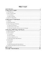
Figure 1.1. The first ‘highresolution’ proton NMR spectrum,
recorded at 30 MHz, displaying the
proton chemical shifts in ethanol
(reprinted with permission from [6],
Copyright 1951, American Institute
of Physics).

High-Resolution NMR Techniques in Organic Chemistry

another through intervening chemical bonds. Although these observations were seen as
unwelcome chemical complications by the investigating physicists, a few pioneering
chemists immediately realised the significance of these chemical shifts and spin–spin
couplings within the context of structural chemistry. The first high-resolution proton
NMR spectrum (Fig. 1.1) clearly demonstrated how the features of an NMR spectrum, in
this case chemical shifts, could be directly related to chemical structure, and it is from this
that NMR has evolved to attain the significance it holds today.
The 1950s also saw a variety of instrumental developments that were to provide the
chemist with even greater chemical insight. These included the use of sample spinning for
averaging to zero field inhomogeneities, which provided a substantial increase in resolution, so revealing fine splittings from spin–spin coupling. Later, spin decoupling was able to
provide more specific information by helping the chemists understand these interactions.
With these improvements, sophisticated relationships could be developed between chemical structure and measurable parameters, leading to realisations such as the dependence of
vicinal coupling constants on dihedral angles (the now well-known Karplus relationship).
The inclusion of computers during the 1960s was also to play a major role in enhancing the

influence of NMR on the chemical community. The practice of collecting the same
continuous wave spectrum repeatedly and combining them with a CAT (computer of
average transients) led to significant gains in sensitivity and made the observation of
smaller sample quantities a practical realisation. When the idea of stimulating all spins
simultaneously with a single pulse of radio frequency, collecting the time-domain response
and converting this to the required frequency-domain spectrum by a process known as
Fourier transformation (FT), was introduced, more rapid signal averaging became possible.
This approach provided an enormous increase in signal-to-noise ratio and was to change
completely the development of NMR spectroscopy. The mid-1960s also saw the application
of the nuclear Overhauser effect (NOE) to conformational studies. Although described
during the 1950s as a means of enhancing the sensitivity of nuclei through the simultaneous
irradiation of electrons, the Overhauser effect has since found widest application in
sensitivity enhancement between nuclei, or in the study of the spatial proximity of nuclei,
and remains one of the most important tools of modern NMR. By the end of the 1960s, the
first commercial FT spectrometer was available, operating at 90 MHz for protons. The next
great advance in field strengths was provided by the introduction of superconducting
magnets during the 1970s, which were able to provide significantly higher fields than the
electromagnets previously employed. These, combined with the FT approach, made the
observation of carbon-13 routine and provided the organic chemists with another probe of
molecular structure. This also paved the way for the routine observation of a whole variety
of previously inaccessible nuclei of low natural abundance and low magnetic moment. It
was also in the early 1970s that the concept of spreading the information contained within
the NMR spectrum into two separate frequency dimensions was proposed in a lecture.
However, because of instrumental limitations, the quality of the first two-dimensional (2D)
spectra was considered too poor to be published, and not until the mid-1970s, when
instrument stability had improved and developments in computers made the necessary
complex calculations feasible, did the development of 2D methods begin in earnest.
These methods, together with the various multipulse one-dimensional (1D) methods that
also became possible with the FT approach, did not have significant impact on the wider
chemical community until the 1980s, from which point their development was nothing less

than explosive. This period saw an enormous number of new pulse techniques presented
that were capable of performing a variety of ‘spin gymnastics’, thus providing the chemist
with ever more structural data, on smaller sample quantities and in less time. No longer was
it necessary to rely on empirical correlations of chemical shifts and coupling constants with
structural features to identify molecules, but instead a collection of spin interactions
(through-bond, through-space and chemical exchange) could be mapped and used to
determine structures more reliably and more rapidly. The evolution of new pulse methods
continued throughout the 1990s, alongside which has emerged a fundamentally different
way of extracting the desired information from molecular systems. Pulsed field gradient
selected experiments have now become routine structural tools, providing better quality
spectra, often in shorter times, than was previously possible. These came into widespread
use not so much from a theoretical breakthrough (their use for signal selection was first
demonstrated in 1980) but again as a result of progressive technological developments
defeating practical difficulties. Similarly, the emergence of coupled analytical methods,
such as liquid chromatography and NMR (LC-NMR), has come about after the experimental complexities of interfacing these very different techniques have been overcome, and
these methods have established themselves for the analysis of complex mixtures. Developments in probe technologies over the last decade have led to the wider adoption of
cryogenically cooled coils in probe heads that reduce significantly system noise and so

www.pdfgrip.com


Chapter 1: Introduction

enhance signal-to-noise ratios. Probe coil miniaturisation has also provided a boost in
signal-to-noise for mass-limited samples, and the marrying of this with cryogenic technology nowadays offers one of the most effective routes to higher detection sensitivity.
Instrument miniaturisation has been a constant theme in recent years leading to smaller
and more compact consoles driven by developments in solid-state electronics. Likewise,
new generations of actively shielded superconducting magnets with significantly reduced
stray fields are now commonplace, making the siting of instruments considerably easier and
far less demanding on space. For example, the first generation unshielded magnets operating at 500 MHz possessed stray fields that would extend to over 3 m horizontally from the

magnet centre when measured at the 0.5 mT (5 gauss) level, the point beyond which
disturbances to the magnetic field are not considered problematic. Nowadays, the latest
generation shielded magnets have this line sited at somewhat less than 1 m from the centre
and only a little beyond the magnet cryostat itself. This is achieved through the use of
compensating magnet coils that seek to counteract the stray field generated outside of the
magnet assembly. Other developments are seeking to recycle the liquid cryogens needed to
maintain the superconducting state of the magnet through the reliquification of helium and
nitrogen. Recycling of helium in this manner is already established for imaging magnets but
poses considerable challenges in the context of high-resolution NMR measurements.
Modern NMR spectroscopy is now a highly developed and technologically advanced
subject. With so many advances in NMR methodology in recent years, it is understandably
an overwhelming task for the research chemist, and even the dedicated spectroscopist, to
appreciate what modern NMR has to offer. This text aims to assist in this task by presenting
the principal modern NMR techniques and exemplifying their application.

1.2. MODERN HIGH-RESOLUTION NMR AND THIS BOOK
There can be little doubt that NMR spectroscopy now represents the most versatile and
informative spectroscopic technique employed in the modern chemical research laboratory
and that an NMR spectrometer represents one of the largest single investments in analytical
instrumentation the laboratory is likely to make. For both these reasons, it is important that
the research chemist is able to make the best use of the available spectrometer(s) and to
harness modern developments in NMR spectroscopy in order to promote their chemical or
biochemical investigations. Even the most basic modern spectrometer is equipped to perform a myriad of pulse techniques capable of providing the chemist with a variety of data
on molecular structure and dynamics. Not always do these methods find their way into the
hands of the practising chemist, remaining instead in the realms of the specialist, obscured
behind esoteric acronyms or otherwise unfamiliar NMR jargon. Clearly, this should not be
so, and the aim of this book is to gather up the most useful of these modern NMR methods
and present them to the wider audience who should, after all, find greatest benefit from their
applications.
The approach taken throughout is non-mathematical and is based firmly on using

pictorial descriptions of NMR phenomena and methods wherever possible. In preparing
and updating this work, I have attempted to keep in mind what I perceive to be the
requirements of three major classes of potential readers:
1. those who use solution-state NMR as tool in their own research, but have little or no
direct interaction with the spectrometer,
2. those who have undertaken training in directly using a spectrometer to acquire their own
data, but otherwise have little to do with the upkeep and maintenance of the instrument,
and
3. those who make use spectrometers and are responsible for the day-to-day upkeep of the
instrument. This may include NMR laboratory managers, although in some cases the
user may not consider themselves dedicated NMR spectroscopists.
The first of these could well be research chemists and students in an academic or
industrial environment who need to know what modern techniques are available to assist
them in their efforts, but otherwise feel they have little concern for the operation of a
spectrometer. Their data is likely to be collected under fully automated conditions or
provided by a central analytical facility. The second may be a chemist in an academic
environment who has hands-on access to a spectrometer and has his or her own samples that
demand specific studies that are perhaps not available from fully automated instrumentation. The third class of reader may work in a smaller chemical company or academic
chemistry department who have invested in NMR instrumentation but may not employ a
dedicated NMR spectroscopist for its upkeep, depending instead on, say, an analytical or
synthetic chemist for this. This, it appears (in the UK at least), is often the case for new

www.pdfgrip.com

3


4

High-Resolution NMR Techniques in Organic Chemistry


start-up chemical companies. NMR laboratory managers may also find the text a useful
reference source. With these in mind, the book contains a fair amount of practical guidance
on both the execution of NMR experiments and the operation and upkeep of a modern
spectrometer. Even if you see yourself in the first of the above categories, some rudimentary understanding of how a spectrometer collects the data of interest and how a sequence
produces, say, the 2D correlation spectrum awaiting analysis on your desk can be enormously helpful in correctly extracting the information it contains or in identifying and
eliminating artefacts that may arise from instrumental imperfections or the use of less than
optimal conditions for your sample. Although not specifically aimed at dedicated spectroscopists, the book may still contain new information or may serve as a reminder of what
was once understood but has somehow faded away. The text should be suitable for (UK)
graduate level courses on NMR spectroscopy, and sections of the book may also be
appropriate for use in advanced undergraduate courses. The book does not, however,
contain descriptions of the basic NMR phenomena such as chemical shifts and coupling
constants, and neither does it contain extensive discussions on how these may be correlated
with chemical structures. These topics are already well documented in various introductory
texts [7–12], and it is assumed that the reader is already familiar with such matters.
Likewise, the book does not seek to provide a comprehensive physical description of the
processes underlying the NMR techniques presented; the book by Keeler [13] presents this
at an accessible yet rigorous level.
The emphasis is on techniques in solution-state (high-resolution) spectroscopy, principally those used throughout organic chemistry as appropriate for this series, although
extensions of the discussions to inorganic systems should be straightforward, relying on
the same principles and similar logic. Likewise, greater emphasis is placed on small to midsized molecules (with masses up to a few thousand say) since it is on such systems that the
majority of organic chemistry research is performed. That is not to say that the methods
described are not applicable to macromolecular systems, and appropriate considerations are
given when these deserve special comment. Biological macromolecules are not covered
however, but are addressed in a number of specialised texts [14–16].

1.2.1. What this book contains
The aim of this text is to present the most important NMR methods used for organic
structure elucidation, to explain the information they provide, how they operate and to
provide some guidance on their practical implementation. The choice of experiments is

naturally a subjective one, partially based on personal experience, but also taking into
account those methods most commonly encountered in the chemical literature and those
recognised within the NMR community as being most informative and of widest applicability. The operation of many of these is described using pictorial models (equations
appear infrequently and are only included when they serve a specific purpose) so that the
chemist can gain some understanding of the methods they are using without recourse to
uninviting mathematical descriptions. The sheer number of available NMR methods may
make this seem an overwhelming task, but in reality, most experiments are composed of a
smaller number of comprehensible building blocks pieced together, and once these have
been mastered, an appreciation of more complex sequences becomes a far less daunting
task. For those readers wishing to pursue a particular topic in greater detail, the original
references are given but otherwise all descriptions are self-contained.
Following this introductory section, Chapter 2 introduces the basic model used throughout the book for the description of NMR methods and describes how this provides a simple
picture of the behaviour of chemical shifts and spin–spin couplings during pulse experiments. This model is then used to visualise nuclear spin relaxation, a feature of central
importance for the optimum execution of all NMR experiments (indeed, it seems early
attempts to observe NMR failed most probably because of a lack of understanding at the
time of the relaxation behaviour of the chosen samples). Methods for measuring relaxation
rates also provide a simple introduction to multipulse NMR sequences. Chapter 3 describes
the practical aspects of performing NMR spectroscopy. This is a chapter to dip into as and
when necessary and is essentially broken down into self-contained sections relating to the
operating principles of the spectrometer and the handling of NMR data, how to correctly
prepare the sample and the spectrometer before attempting experiments, how to calibrate
the instrument and how to monitor and measure its performance, should you have such
responsibilities. It is clearly not possible to describe all aspects of experimental spectroscopy in a single chapter, but this (together with some of the descriptions in Chapter 10)
should contain sufficient information to enable the execution of most modern experiments.
These descriptions are kept general, and in these, I have deliberately attempted to avoid the
use of a dialect specific to a particular instrument manufacturer. Chapter 4 contains the

www.pdfgrip.com



Chapter 1: Introduction

most widely used 1D techniques, ranging from the optimisation of the single-pulse experiment to the multiplicity editing of heteronuclear spectra and the concept of polarisation
transfer, another feature central to pulse NMR methods. This includes the universally
employed methods for the editing of carbon spectra according to the number of attached
protons. Specific requirements for the observation of certain quadrupolar nuclei that posses
extremely broad resonances are also considered. The introduction of 2D methods is presented in Chapter 5, specifically in the context of determining homonuclear correlations.
This is so that the 2D concept is introduced with a realistically useful experiment in mind,
although it also becomes apparent that the general principles involved are common to any
2D experiment. Following this, a variety of correlation techniques are presented for
identifying scalar (J) couplings between homonuclear spins, which for the most part
means protons although methods for correlating spins of low abundance nuclides such as
carbon are also discussed. Included in this chapter is an introduction to the operation and
use of pulsed field gradients, again with a view to presenting them with a specific
application in mind. Again, these discussions aim to make clear that the principles involved
are quite general and can be applied to a variety of experiments. Those that benefit most
from the gradient methodology are the heteronuclear correlation techniques given in
Chapter 6. These correlations are used to map coupling interactions between, typically,
protons and a heteroatom either through a single bond or across multiple bonds. In this
chapter, most attention is given to the modern correlation methods based on proton
excitation and detection, so-called ‘inverse’ spectroscopy. These provide significant gains
in sensitivity over the traditional methods that use detection of the less sensitive heteroatom, which nevertheless warrant description because of specific advantages they provide
for certain molecules. Chapter 7 considers methods for separating chemical shifts and
coupling constants in spectra, which are again based on 2D methods. Chapter 8 moves
away from through-bond couplings and onto through-space interactions in the form of the
NOE. The principles behind the NOE are presented initially for a simple two-spin system,
and then for more realistic multi-spin systems. The practical implementation of both 1D and
2D NOE experiments is described, including the widely used pulsed field gradient 1D NOE
methods. Rotating-frame NOE (ROE) techniques are also described, which find greatest
utility in the study of larger molecules for which the NOE can be poorly suited, having

application in studies of host–guest complexes, oligomeric structures, supramolecular
systems and so on. Chapter 9 extends into the study of self-diffusion, an area now routinely
amenable to investigation on spectrometers equipped with standard pulsed field gradient
hardware. This presents a new chapter for the second edition and reflects the wider use of
diffusion NMR methods to studies of a variety of molecular interactions in solution, to the
investigation of mixtures and to the classification of molecular size. The final chapter
considers additional experimental methods that do not, on their own, constitute complete
NMR experiments but are the tools with which modern methods are constructed. These are
typically used as elements within the sequences described in the preceding chapters and
include such topics as broadband decoupling, selective excitation of specific regions of a
spectrum and solvent suppression. Finally, the chapter concludes with a brief overview of
some emerging methods, including an approach to very fast 2D data acquisition, new
methodology for boosting detection sensitivity and an alternative approach to defining
stereochemistry in small organic molecules. At the end of the book is a glossary of some of
the acronyms that permeate the language of modern NMR, and, it might be argued, have
come to characterise the subject. Whether you love them or hate them they are clearly here
to stay and although they provide a ready reference when speaking of pulse experiments to
those in the know, they can also serve to confuse the uninitiated and leave them bewildered
in the face of this NMR jargon. The glossary provides an immediate breakdown of the
acronym together with a reference to its location in the book.

1.2.2. Pulse sequence nomenclature
Virtually all NMR experiments can described in terms of a pulse sequence, which, as the
name suggests, is a notation which describes the series of radiofrequency (rf) or fieldgradient pulses used to manipulate nuclear spins and so tailor the experiment to provide the
desired information. Over the years, a largely (although not completely) standard pictorial
format has evolved for representing these sequences, not unlike the way a musical score is
used to encode a symphony1. As these crop up repeatedly throughout the text, the format
and conventions used in this book deserve explanation. Only the definitions of the various

1


Indeed, just as a skilled musician can read the score and ‘hear’ the symphony in his head, an experienced
spectroscopist can often read the pulse sequence and picture the general form of the resulting spectrum.

www.pdfgrip.com

5


6

High-Resolution NMR Techniques in Organic Chemistry
a)
90x°

180x°

Δ

nuclide 1

Radiofrequency
pulses

90x°

90x°

t1


nuclide 2

G1

Field gradient
pulses

(Decouple)
G2

G3

z-axis

b)

x
1H

x

Δ

Δ
x

Figure 1.2. Pulse sequence
nomenclature. (a) A complete pulse
sequence and (b) the reduced
representation used throughout the

remainder of the book.

t2(x)

Δ

x

x

X

t1
G1

(Decouple)
G2

G3

Gz

pictorial components of a sequence are given here, their physical significance in an NMR
experiment will become apparent in later chapters.
An example of a reasonably complex sequence is shown in Fig. 1.2 (a heteronuclear
correlation experiment from Chapter 6), and it illustrates most points of significance.
Figure 1.2a represents a more detailed account of the sequence, whilst Fig. 1.2b is the
reduced equivalent used throughout the book for reasons of clarity. The rf pulses applied to
each nuclide involved in the experiment are presented on separate rows running left to right,
in the order in which they are applied. Most experiments nowadays involve protons, and

often one (and sometimes two) other nuclides as well. In organic chemistry, this is naturally
most often carbon but can be any other, so is termed the X-nucleus. These rf pulses are most
frequently applied as so-called 90° or 180° pulses (the significance of which is detailed in
the following chapter), which are illustrated by a thin black bar and thick grey bars,
respectively (Fig. 1.3). Pulses of other angles are marked with an appropriate Greek symbol
that is described in the accompanying text. All rf pulses also have associated with them a
particular phase, typically defined in units of 90° (0°, 90°, 180°, 270°), and indicated above
each pulse by x, y, –x or –y, respectively. If no phase is defined, the default will be x. Pulses
that are effective over only a small frequency window and act only on a small number of
resonances are differentiated as shaped rather than rectangular bars as this reflects the
manner in which these are applied experimentally. These are the so-called selective or
shaped pulses described in Chapter 10. Pulses that sweep over very wide bandwidths are
indicated by horizontal shading to reflect the frequency sweep employed, as also explained
in the final chapter. Segments that make use of a long series of very many closely spaced
pulses, such as the decoupling shown in Fig. 1.2, are shown as a solid grey box, with the
bracket indicating the use of the decoupling sequence is optional. Below the row(s) of rf
pulses are shown field gradient pulses (Gz), whenever these are used, again drawn as shaped
pulses where appropriate, and shown greyed when considered optional elements within a
sequence.

Radio frequency pulses
90° high-power (hard) pulse

Shaped gradient pulse

180° high-power (hard) pulse

Gradient gated on-off

Low-power pulse or train of pulses


Incremented gradient sequence

Shaped low-power (soft) pulse

Figure 1.3. A summary of the pulse
sequence elements used throughout
the book.

Field gradient pulses

Frequency swept (adiabatic) pulse

www.pdfgrip.com

Free Induction Decay

Data acquisition period


Chapter 1: Introduction

The operation of very many NMR experiments is crucially dependent on the experiment
being tuned to the value of specific coupling constants. This is achieved by defining certain
delays within the sequence according to these values; these delays being indicated by the
general symbol D. Other time periods within a sequence that are not tuned to J-values but
are chosen according to other criteria, such as spin recovery (relaxation) rates, are given the
symbol . The symbols t1 and t2 are reserved for the time periods, which ultimately
correspond to the frequency axes f1 and f2 of 2D spectra, one of which (t2) will always
correspond to the data acquisition period when the NMR response is actually detected. The

acquisition period is illustrated by a simple decaying sine wave in all experiments to
represent the so-called free induction decay (FID). Again it should be stressed that although
these sequences can have rather foreboding appearances, they are generally built up from
much smaller and simpler segments that have well-defined and easily understood actions.
A little perseverance can clarify what might at first seem a total enigma.

1.3. APPLYING MODERN NMR TECHNIQUES
The tremendous growth in available NMR pulse methods over the last three decades can
be bewildering and may leave one wondering just where to start or how best to make use of
these new developments. The answer to this is not straightforward since it depends so much
on the chemistry undertaken, on the nature of the molecule being handled and on the
information required of it. It is also dependent on the amount of material and on the
available instrumentation and its capabilities. The fact that NMR itself finds application
in so many research areas means defined rules for experiment selection are largely
intractable. A scheme that is suitable for tackling one type of problem may be wholly
inappropriate for another. Nevertheless, it seems inappropriate that a book of this sort
should contain no guidance on experiment selection other than the descriptions of the
techniques in the following chapters. Here I attempt to broach this topic in rather general
terms and present some loose guidelines to help weave a path through the maze of available
techniques. Even so, only with a sound understanding of modern techniques can one truly
be in a position to select the optimum experimental strategy for your molecule or system,
and it is this understanding I hope to develop in the remaining chapters.
Most NMR investigations will begin with the analysis of the proton spectrum of the
sample of interest, with the usual analysis of the chemical shifts, coupling constants and
relative signal intensities, either manually or with the assistance of the various sophisticated
computer-based structure spectrum databases now available. Beyond this, one encounters a
plethora of available NMR methods to consider employing. The key to selecting appropriate experiments for the problem at hand is an appreciation of the type of information the
principal NMR techniques can provide. Although there exist a huge number of pulse
sequences, there are a relatively small number of what might be called core experiments,
from which most others are derived by minor variation, of which only a rather small

fraction ever find widespread use in the research laboratory. To begin, it is perhaps
instructive to realise that the NMR methods presented in this book exploit four basic
phenomena:
1. Through-bond interactions: scalar (J) spin coupling via bonding electrons.
2. Through-space interactions: the NOE mediated through dipole–dipole coupling and spin
relaxation.
3. Chemical exchange: the physical exchange of one spin for another at a specific location.
4. Molecular self-diffusion: the translational movement of a molecule or complex.
When attempting to analyse the structure of a molecule and/or its behaviour in solution
by NMR spectroscopy, one must therefore consider how to exploit these phenomena to gain
the desired information, and from this select the appropriate technique(s). Thus, when
building up the structure of a molecule, one typically first searches for evidence of scalar
coupling between nuclei as this can be used to indicate the location of chemical bonds.
When the location of all bonding relationships within the molecule has been established, the
gross structure of the molecule is defined. Spatial proximities between nuclei, and between
protons in particular, can be used to define stereochemical relationships within a molecule
and thus address questions of configuration and conformation. The unique feature of NMR
spectroscopy, and the principal reason for its superiority over any other solution-state
technique for structure elucidation, is its ability to define relationships between specific
nuclei within a molecule or even between molecules. Such exquisite detail is generally
obtained by correlating one nucleus with another by exploiting the above phenomena.
Despite the enormous power of NMR, there are, in fact, rather few types of correlation
available to the chemist to employ for structural and conformational analysis. The principal

www.pdfgrip.com

7


High-Resolution NMR Techniques in Organic Chemistry


8

Table 1.2. The principal correlations or interactions established through NMR techniques. The correlated spins are shown in bold type for each
correlation, with X indicating any spin-½ nucleus. The acronyms are explained in the glossary
Correlation

Principal technique(s)

Comments

H

1

Proton J-coupling typically over two or three bonds

5

1

Relayed proton J-couplings within a coupled spin system. Remote protons may be
correlated provided there is a continuous coupling network in between them

5

1

One-bond heteronuclear couplings with proton observation


6

1

Long-range heteronuclear couplings with proton observation. Typically over two or three
bonds when X = 13C

6

X–X COSY
X–X INADEQUATE
H–X–X–H
ADEQUATE

COSY only used when X spin natural abundance is greater than 20%. Sensitivity
problems when X has low natural abundance; can be improved with proton detection
methods

5

1
H–1H NOE difference
1/2D NOESY
1/2D ROESY

Through-space correlations. NOE difference only applicable to ‘small’ molecules,
ROESY applicable to ‘mid-sized’ molecules with masses of ca. 1–2 kDa

8


1
H–X NOE difference
2D HOESY

Sensitivity limited by X spin observation. Care required to make NOEs specific in
presence of proton decoupling

8

1D saturation or
inversion transfer
2D EXSY

Interchange of spins at chemically distinct locations. Exchange must be slow on NMR
timescale for separate resonances to be observed. Intermediate to fast exchange requires
lineshape analysis

8

Spin-echo or
stimulated-echo
methods
2D DOSY

Measurement of molecular self-diffusion using pulsed field gradient technology. Used
mainly in studies of molecular associations

9

X

H

X
H

J

X

H

X

H
J
X

X

NOE

H

H–X HMQC
H–X HSQC

X
NOE

H

X

Exchange
A

X

X
J

X

H–1H TOCSY

H–X HMBC

X

X

H

J

X

H

J


1

X
H

H–1H COSY

H

J

Chapter

B

Diffusion

1D, one-dimensional; 2D, two-dimensional; NOE, nuclear Overhauser effect.

spin interactions and the main techniques used to map these, which are frequently 2D
methods, are summarised in Table 1.2 and further elaborated in the chapters that follow.
The homonuclear correlation experiment, correlation spectroscopy (COSY), identifies
those nuclei that share a J-coupling, which, for protons, operate over two, three and, less
frequently, four bonds. This information can therefore be used to indicate the presence of a
bonding pathway. The correlation of protons that exist within the same coupled network or
chain of spins, but do not themselves share a J-coupling, can be made with the total
correlation spectroscopy (TOCSY) experiment. This can be used to identify groups of
nuclei that sit within the same isolated spin system, such as the amino acid residue of a
peptide or the sugar ring of an oligosaccharide. One-bond heteronuclear correlation methods (heteronuclear multiple-quantum correlation (HMQC) or heteronuclear single-quantum
correlation (HSQC)) identify the heteroatoms to which the protons are directly attached and

can, for example, provide carbon assignments from previously established proton assignments. Proton chemical shifts can also be dispersed according to the shift of the attached
heteroatom, so aiding the assignment of the proton spectrum itself. Long-range heteronuclear correlations over typically two or three bonds (heteronuclear multiple-bond correlation (HMBC)) provide a wealth of information on the skeleton of the molecule and can be
used to infer the location of carbon–carbon or carbon–heteroatom bonds. These correlations
can be particularly valuable when proton–proton correlations are absent. The incredible
natural abundance double quantum transfer experiment (INADEQUATE)-based experiments identify connectivity between like nuclei of low natural abundance, for which it is
favoured over COSY. This can therefore correlate directly connected carbon centres, but as

www.pdfgrip.com


Chapter 1: Introduction

9

this relies on the presence of neighbouring carbon-13 nuclei, it suffers from appallingly low
sensitivity and thus finds little use. Modern variants that use proton detection, termed
adequate sensitivity double-quantum spectroscopy (ADEQUATE), have greatly improved
performance but are still less used than the heteronuclear correlation techniques. Measurements based on the NOE are most often applied after the gross structure is defined, and NMR
assignments established, to define the three-dimensional (3D) stereochemistry of a molecule
since these effects map through-space proximity between nuclei. It can also provide insights
into the conformational folding of larger structures and the direct intermolecular interactions.
The vast majority of these experiments investigate proton–proton NOEs, although in exceptional cases, heteronuclear NOEs involving a proton and a heteroatom have been applied
successfully. Similar techniques to those used in the observation of NOEs can also be
employed to correlate nuclei involved in chemical exchange processes that are slow on the
NMR timescale and so give rise to distinct resonances for each exchanging species or site.
Finally, methods for the quantification of molecular self-diffusion provide information on the
nature and extent of molecular associations and provide a complimentary view of solution
behaviour. They may also be used to separate the spectra of species with differing mobilities
and have potential application in the characterisation of mixtures.
The greatest use of NMR in the chemical research laboratory is in the routine characterisation of synthetic starting materials, intermediates and final products. In these circumstances, it is often not so much full structure elucidation that is required, rather it is structure

confirmation or verification since the synthetic reagents are known, which naturally limit
what the products may be, and because the desired synthetic target is usually defined.
Routine analysis of this sort typically follows a general procedure similar to that summarised in Table 1.3, which is supplemented with data from the other analytical techniques,
most notably mass spectrometry and infrared spectroscopy. The execution of many of the
experiments in Table 1.3 benefits nowadays from the incorporation of pulsed field gradients
to speed data collection and to provide spectra of higher quality. Furthermore, experiments
involving heteronuclear correlations typically employ proton observation to aid sensitivity
rather the detection of the heteronuclide as was the case for earlier 2D methods. Nowadays,
the collection of a 2D proton-detected 1H–13C shift correlation experiment requires significantly less time than the 1D carbon spectrum of the same sample, providing both carbon
shift data (of protonated centres) and correlation information. This can be a far more
powerful tool for routine structure confirmation than the 1D carbon experiment alone. In
addition, editing can be introduced to the 2D experiment to differentiate methine from
methylene correlations for example, providing yet more data in a single experiment and in
less time. Even greater gains can be made in the indirect observation of heteronuclides of
still lower intrinsic sensitivity, for example, nitrogen-15, and when considering the observation of low abundance nuclides it is sensible to first consider adopting a proton-detected
method for this. The structure confirmation process can also be enhanced through the
measured use of spectrum prediction tools that are now widely available. The generation
Table 1.3. A typical protocol for the routine structure confirmation of synthetic organic materials. Not all these steps may be necessary, and the direct
observation of a heteronuclide, such as carbon or nitrogen, can often be replaced through its indirect observation with the more sensitive protondetected heteronuclear shift correlation techniques
Procedure

Technique

Information

1D 1H spectrum
Œ

1D


Information from chemical shifts, coupling constants, integrals

2D 1H–1H correlation
Œ

COSY

Identify J-coupling relationships between protons

1D 13C (with spectrum editing)

1D, (DEPT or
APT)

Carbon count and multiplicity determination (C, CH, CH2, CH3). Can often be avoided
by using proton-detected heteronuclear 2D experiments

1D heteronuclide spectra
e.g. 31P, 19F
Œ

1D

Chemical shifts and homonuclear/heteronuclear coupling constants

2D 1H–13C one-bond correlation
(with spectrum editing)
Œ

HMQC or HSQC

(with editing)

13

2D 1H–13C long-range correlation

HMBC

Correlations identified over two and three bonds. Correlations established across
heteroatoms, e.g. N and O. Fragments of structure pieced together

1D or 2D NOE

Stereochemical analysis: configuration and conformation

Œ

Carbon assignments transposed from proton assignments. Proton spectrum dispersed by
C shifts. Carbon multiplicities from edited HSQC (faster than above 1D approach)

Œ
Through-space NOE correlation

1D, one-dimensional; 2D, two-dimensional; NOE, nuclear Overhauser effect.

www.pdfgrip.com