3.1
Macro-geometric Features
A. Weckenmann, Universität Erlangen-Nürnberg, Erlangen, Germany
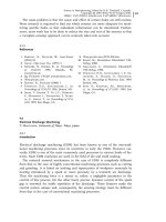
Measurement of macro-geometric characteristic variables involves the acquisition
of features of geometric elements that are defined in design by dimensions and
tolerances for dimensional, form, and positional deviations (Figure 3.1-1). The
term ‘dimension’ refers both to the diameter of rotationally symmetrical work-
pieces and to distances and angles between planes and straight lines and to cone
angles.
The sensors used for measurement can be classified according to the method
used to acquire the measured value into mechanical, electrical, and optoelectronic
sensors. A small proportion work by other methods, eg, pneumatic measuring
methods.
The sensors mainly work with point-by-point, usually tactile measured value ac-
quisition. Contactless and wide-area measurements of characteristic variables of
the rough shape are possible with optical sensors.
71
3
Sensors for Workpieces
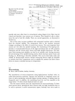
Fig. 3.1-1 Deviations of the macro
shape of workpieces
Sensors in Manufacturing. Edited by H.K. Tönshoff, I. Inasaki
Copyright © 2001 Wiley-VCH Verlag GmbH
ISBNs: 3-527-29558-5 (Hardcover); 3-527-60002-7 (Electronic)
3.1.1
Mechanical Measurement Methods
By far the greatest number of measuring systems used in dimensional metrology
work with tactile probes and mechanical transmission of the measured value. For
acquisition and indication of the measured value, a linear scale is usually used or
the measured value is transmitted to deflection of a needle, say, by means of a
rack and pinion. Indication is analog. Measuring instruments with a digital dis-

play usually use measuring systems with capacitive, inductive, or optoelectronic
(Section 3.1.4) measured value acquisition.
3.1.1.1 Calipers
The various designs of calipers (DIN 862) are used for outside, inside, and depth
measurements. The measured length is transmitted mechanically and a scale with
millimeter divisions that can be read absolutely is used. Use of a Vernier scale
provides an additional means of displaying 1/10, 1/20, or 1/50 mm graduations
(Figure 3.1-2). The function, eg, of the 1/10 mm Vernier scale, is based on provid-
ing a length of 39 mm with 10 graduation marks at equal intervals. The point at
which a graduation mark on the main scale is aligned with a graduation mark on
the Vernier scale indicates the number of 1/10 mm on the measured length.
Sometimes a division with 20 graduation marks or a rotary dial is used instead of
the Vernier scale with 10 graduation marks.
Except for the depth gage, the scale of a caliper and the measuring object can-
not be fully aligned. This violation of Abbe’s comparator principle causes a sine de-
viation between the scale and the slider due to an angular deviation (Figure 3.1-3,
Table 3.1-1). When expanding into a Taylor series, the angle of the tilt is included
linearly in the result error. We therefore refer to it as a first-order error.
3 Sensors for Workpieces72
Fig. 3.1-2 Vernier caliper
3.1.1.2 Protractors
A measuring instrument which works in an analogous way to the caliper is the
universal protractor for measuring angles (Figure 3.1-4). The universal protractor
also has an absolute angular scale and a Vernier scale, which allows the user to
read off angular dimensions in steps of 5'. Models with a digital display are also
available. Their smallest graduation is 1'.
3.1.1.3 Micrometer Gages
Some types of micrometer gages (DIN 863) can be used for the same tasks as cali-
pers. Micrometer calipers (Figure 3.1-5) are used for outside measurements and
inside measurements (measuring range usually about 25 mm) and depth micro-

meters for depth measurements. Drill-hole diameters can be measured using
three-point inside micrometer gages.
A threaded spindle is used to transfer the measured value to the scale on the
sleeve. The graduations on the sleeve indicate steps, each of which corresponds to
one turn of the threaded spindle. A further, finer subdivision is also marked on a
circumferential division on the scale thimble. The scale interval is usually 0.01
mm. A slip clutch ensures that the measuring force is limited. Insulation ensures
3.1 Macro-geometric Features 73
Fig. 3.1-3 Violation of the comparator
principle on a caliper
Tab. 3.1-1 Sine deviation for a measuring arm length l =40 mm
Angular deviation, u
1' 5' 10' 1 8
Sine deviation, f (lm) 11.6 58.2 116.4 698.1
Fig. 3.1-4 Universal protractor (courtesy: Brown and Sharpe)
that heat from the hands is not transferred to the measuring instruments, which
could otherwise cause a thermally induced alteration in length.
Special inserts for the fixed anvil and the measuring surface of the spindle per-
mit an extension of the application range. For example, if a notch and cone are
used, it is possible to measure flank diameters on threads, and larger measuring
contacts are used to measure tooth widths. Models with numerical or digital dis-
plays also exist.
Micrometer gages ensure that the measuring object and the scale are aligned.
Since the comparator principle is not violated, no first-order measuring error can
occur; only a second-order error remains (also called a cosine deviation, Fig-
ure 3.1-6), which is much less significant (Table 3.1-2). According to the measur-
ing range, the maximum total discrepancy span is specified between 4 and 13 lm
(DIN 863-1).
3 Sensors for Workpieces74
Fig. 3.1-5 Micrometer caliper

with measuring head
Fig. 3.1-6 Cosine deviation in measure-
ment using a micrometer caliper
3.1.1.4 Dial Gages
With their comparatively short plunger travel (3 or 10 mm), dial gages (Fig-
ure 3.1-7a, DIN 878) are mostly used for differential measurements. Their applica-
tions are checking straightness, parallelism, or circularity. To determine an abso-
lute dimension with a dial gage and stand, it is first necessary to set the required
specified dimension with a material measure, say, a parallel gage block, and then
to adjust the needle to a defined deflection (calibration).
The displacement of the measuring bolt is transmitted to a gear-wheel mecha-
nism via a rack, converting the distance measured to needle deflection. The result
is displayed on a circumferential scale with a scale interval of typically 0.01 mm.
Since dial gages indicate a width of backlash, measurements should be performed
only touching the measuring object in the same direction as when calibrating. Ra-
dial run-out measurements can therefore be afflicted with systematic errors. On
dial gages, the needle can revolve around the scale several times over the entire
plunger travel; a small pointer then counts the number of revolutions. Dial gages
are also available in digital versions. The probe tip diameter is usually 3 mm, but
numerous other probe styluses are available, eg, pointed, cutting edge, plane or
ball measuring contacts, balls of other diameters, or measuring rollers. According
to the measuring range, the maximum total discrepancy span is specified between
9 and 17 lm (DIN 878).
3.1 Macro-geometric Features 75
Tab. 3.1-2 Cosine deviation for spindle length d =20 mm
Angular deviation, u
1' 5' 10' 1 8
Cosine deviation, f ( lm) 0.001 0.021 0.85 3.046
a) Dial gage b) Comparator dial c) Lever-type test
indicator

Fig. 3.1-7 Dial gage, comparator dial, and lever-type test indicator (courtesy: Mahr)
3.1.1.5 Dial Comparators
Dial comparators (Figure 3.1-7b) are also mainly used for differential measure-
ments, but the measuring range is smaller than that of dial gages, usually under
1 mm, with a smaller scale interval, starting at 0.5 lm according to the standards
(DIN 879-1, DIN 879-3). The needle deflection only extends over the angular
range of the scale, and the motion of the measuring bolt is transmitted to the
point via a lever mechanism or a torsion spring, indicating a negligible width of
backlash. Comparator dials with contact limits are used, for example, to indicate
violation of tolerance ranges with a special display unit. The maximum total dis-
crepancy span is specified as 1.2 times the scale interval (DIN 879-1).
3.1.1.6 Lever-type Test Indicators
Lever-type test indicators (Figure 3.1-7 c, DIN 2270) are similar to comparator dials
in both form and function. The angular deflection of the stylus is also transmitted
to the needle via a lever mechanism. A circumferential scale with a scale interval
of 0.002 mm is used for display. The measuring range is smaller than 1 mm.
Although lever-type test indicators use a circumferential scale, unlike on a dial
gage, multiple revolutions of the needle around the scale are not recorded with an
additional small needle. The admissible deviation is specified.
3.1.2
Electrical Measuring Methods
Electrical dimensional measurement has clear advantages over mechanical methods:
· low measuring forces;
· small dimensions of the measured value pickup;
· separation of the measured value pickup and the display unit;
· simple amplification and combination of measuring signals;
· possibility of electrical further processing of the measured length;
· easy connection to a computer and data processing.
This is offset by a greater handling effort.
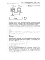
It is possible to distinguish between three types of electrical dimensional mea-

surement (Figure 3.1-8):
3 Sensors for Workpieces76
Fig. 3.1-8 Working principle of electrical dimensional measurements
· resistive displacement sensors;
· capacitive displacement sensors;
· inductive displacement sensors.
A length can be acquired either continuously and analog or incrementally. In in-
cremental systems, numerous basic measuring elements (eg, magnets) are ar-
ranged consecutively at defined intervals on a scale and the number of zero cross-
ings that the measuring bolt produces in the measured signal as it passes the
measuring elements is counted. The measured value is therefore digitized. Com-
mon incremental methods of electrical dimensional measurement function mag-
netically, capacitively, or inductively. What all incremental measured value sensors
have in common is a reference mark that they require to permit absolute mea-
surements. The incrementally determined intervals then refer to this reference
mark which is approached as soon as the instrument is switched on.
3.1.2.1 Resistive Displacement Sensors
Resistive displacement sensors in the form of potentiometers permit the measure-
ment of lengths and angles. The resistance is varied in direct proportion to the
linear or angular displacement via a sliding contact. The voltage, which depends
on the resistance, is measured (Figure 3.1-9). Given a sufficiently high input resis-
tance in the voltmeter, the following applies:
U
a

s
s
0
Á U
0

or U
a

u
u
0
Á U
0
: 3:1-1
Resistance displacement pickups are available with a wound resistance wire on an
insulating main body, or with a continuous resistive layer applied to a material
substrate. The disadvantage is the wear on the sliding contact.
3.1.2.2 Capacitive Displacement Sensors
Capacitive displacement measurement makes use of the effect that the capaci-
tance of a plate capacitor depends on the distance between the capacitor plates.
3.1 Macro-geometric Features 77
Fig. 3.1-9 Potentiometer length and angle measurement
On electrically conductive workpieces, contactless measurement is possible; the
surface of the workpiece is then used as a moveable capacitor plate itself. The ad-
vantage lies in the almost inertialess measured value acquisition which, for exam-
ple, permits circular or axial measurement on cylindrical parts rotating at high
speed. One of its applications is therefore in-process monitoring of spindles in
machine tools. On workpieces with insufficient electrical conductivity, the dimen-
sional measurement has to be transmitted to a moving capacitor plate via a rigid
measuring bolt.
If all the capacitor plates of a capacitive displacement sensor used in the differ-
ential method are identical, it is possible to measure voltage U
a
depending on
length s (Figure 3.1-10 shows a setup of a capacitive displacement sensor). The fol-

lowing applies:
U
a

s
2s
0
Á U
0
: 3:1-2
In dimensional measurement, capacitive displacement sensors are actually used
fairly rarely. They have become common as filling level meters and for the con-
tactless measurement of material thicknesses.
3.1.2.3 Inductive Displacement Sensors
Most electrical dimensional measurement sensors function inductively, there
being two different types of inductive displacement sensors: the plunger core sen-
sor, in which the inductance of a coil varies as a function of the length measured,
and the transformer sensor, in which the transformational coupling between two
coils varies as a function of the length measured.
Inductive probes make use of the effect that in a coil carrying AC, an AC volt-
age is induced having the opposite polarity to the excitation voltage. The magni-
tude of the voltage depends on the inductance of the coil. This inductance can be
varied by moving a magnetic core (plunger core) in the magnetic field of a coil.
Because the inductance measurable via the induction voltage depends on the dis-
placement of the magnetic core in a nonlinear way, the coils are connected in a
differential circuit on inductive probes that produce an output signal that depends
linearly on the displacement of the magnetic core after phase-dependent rectifica-
tion. Two different types of probes are in common use: half-bridge probes on the
plunger core sensor principle and LVDT probes on the transformer sensor princi-
ple (Figure 3.1-11).

3 Sensors for Workpieces78
Fig. 3.1-10 Capacitive displacement sensors
in the differential method
On half-bridge probes (Figure 3.1-12), both coils are directly fed an AC voltage
of approximately 10 kHz. For the measurement signal, the ferrite core functions
as a voltage divider. For the measured induction voltage U
a
the following applies:
U
a

1
2K
Á
DL
L
Á U
0
3:1-3
where DL is proportional to the displacement s and K is a constant. If the plunger
core is precisely in the center between the two coils, the induction voltage is zero.
The induction voltage increases if the plunger core is moved out of the central
position toward one of the two coils. The maximum value is present if only one
coil is completely covered by the plunger core. If it is moved further along the
coil in the same direction, the induction voltage decreases again. The linearity
3.1 Macro-geometric Features 79
Fig. 3.1-11 Working principles of inductive probes
Fig. 3.1-12 Design of an inductive half-bridge probe (courtesy: TESA)
range in which the measurement signal is directly proportional to the displace-
ment of the plunger core is smaller than and included in the unambiguity range

(Figure 3.1-13).
LVDT probes, on the other hand, have one primary coil and two secondary coils
that are arranged concentrically around the moveable plunger core. The primary
coil receives an AC voltage of approximately 5 kHz that is transmitted to the sec-
ondary coils in phase opposition. The measurement signal U
a
derived from the
differential connection of the two secondary coils is directly proportional to the
displacement s of the measuring bolt. The following applies:
U
a
 K Á s Á U
0
: 3:1-4
Inductive displacement sensors can be operated with very small measuring forces
(down to 0.02 N) on some types. Resolutions down to 0.01 lm and small linearity
errors of below 1% permit high-precision dimensional measurements. They are
also suitable for static and dynamic measurements. They are frequently used in
multi-gaging measuring instruments and automatic measuring machines. When
using inductive probes, the thermally induced zero point drift in lm/K, stating
how the measured value indicated varies as a function of the temperature for a
constant measured quantity, must be taken into account.
Eddy current measurement is a special case of inductive dimensional measure-
ment, which is suitable for contactless distance measurement, if the workpiece
material is electrically conductive. If a coil that forms a magnetic field is brought
close to an electrically conductive body, eddy currents form within it which, in
turn, form a magnetic flux with opposite polarity. This causes a reduction in in-
ductance in the coil, which is electrically measurable. The change in inductance
depends on the distance between the coil and the measuring object. For eddy cur-
rent sensors in a differential circuit, a linear relationship is established between

the distance and the change in inductance.
3 Sensors for Workpieces80
Fig. 3.1-13 Unambiguity and linearity
of the measurement signal of an inductive
displacement sensor
3.1.2.4 Magnetic Incremental Sensors
Incremental measuring systems based on magnets use a scale with permanent
magnets as a material measure. The magnets are attached to the scale with alter-
nating opposite polarity. The reading is obtained using ferromagnetic heads into
which an excitation current with a defined frequency is injected.
Depending on the position of the magnetic poles of the reading head with re-
spect to the permanent magnets in the scale, a different voltage will be generated
at the output coils. If the poles of the magnet head are precisely symmetrical with
respect to one pole of the scale, the magnetic fluxes produced by the excitation
coil are shorted. In that case, no signal is present at the output coil. However, if
the two pole shoes are precisely in the center between a north and a south pole of
the scale, induction is caused in the output coil with double the frequency of the
excitation current (Figure 3.1-14). Because of the different responses of the read-
ing head to different positions with respect to the magnetic scale, it is possible to
count how many period lengths of the individual permanent magnets are passed
during motion along the scale. The direction of motion can be detected if two
magnet heads are used for reading, which are arranged such that the measure-
ment signal determined at the same time has a phase offset of one fourth of a
period length. The direction of motion can be determined from the time se-
quence of the signal progressions between the heads.
3.1.2.5 Capacitive Incremental Sensors
Capacitive incremental sensors use scales on which a graduation of thin metal foil
is attached. An identical metal foil is attached to the measuring element opposite
the scale, so that the measuring element and scale together act as a capacitor. If
the measuring element moves along the scale, the capacitance varies sinusoidally.

It is possible to derive the number of graduation periods passed from the number
of zero crossings. Additional interpolation of the sinusoidal signal permits resolu-
tions up to 0.1 lm. Here, too, it is possible to detect the direction of movement
by the fact that a second division is offset by a fourth of the graduation period.
Capacitive incremental scales are used in calipers and micrometer calipers. The
low energy requirement permits uninterrupted use of the measuring instrument
with a battery for about 1 year.
3.1 Macro-geometric Features 81
Fig. 3.1-14 Working principle of magnetic
incremental linear measuring systems
3.1.2.6 Inductive Incremental Sensors
The best known example of an inductive incremental sensor is the inductosyn.
Depending on the type, inductosyn measuring systems can be used for angular
measurement (rotary inductosyn) or displacement measurement (linear inducto-
syn). A meandering conductor path is applied to a nonmagnetic, flat substrate
material, eg, made of glass by means of an etching process. A scale with the re-
quired measurement length and a shorter, moveable cursor, on which two sepa-
rate conductor paths offset by one fourth of a division period are the basic struc-
ture of an inductosyn (Figure 3.1-15).
An alternating voltage is applied to the conductor path of the scale. This induces a
voltage in the conductor paths on the cursor according to the transformer principle.
The amplitude of the induced voltage depends on the relative positions of the con-
ductor paths on the scale and cursor. If the two paths coincide exactly, the amplitude
of the induced voltage is at a maximum. If the conductor path of the cursor is pre-
cisely in the gap between the conductor paths of the scale, no induction occurs (Fig-
ure 3.1-16). The measurement signals are evaluated in an analogous way to the
methods described above for magnetic and capacitive incremental sensors.
The inductosyn is frequently used for positioning in machine tools because it is
largely insensitive to dirt, contrary to optoelectronic measurement methods de-
3 Sensors for Workpieces82

Fig. 3.1-15 Design of the linear inductosyn
Fig. 3.1-16 How the measurement signal
is obtained in an inductosyn
scribed below. On linear guideways it allows almost any measurement length by
adjoining several scales. With a pole pitch of typically 1–2 mm, resolutions down
to 1 lm can be achieved.
3.1.3
Electromechanical Measuring Methods
Each modern coordinate measuring machine (CMM) needs at least one sensing
device for the workpiece data acquisition. Originally, sets of hard probes (spheres,
cones, disk, and cylinders) were the only probes available for use with a CMM.
Different probe tips are shown in Figure 3.1-17.
Today, electromechanical devices are used exclusively. The structure of such a sen-
sing device system is crucial for the measuring accuracy of the CMM, which is ap-
propriate within the range from a few lm to 0.1 lm. Today’s touch trigger probe are
always afflicted by their geometric structure with a first-order error (violation of the
Abbé principle, triangle characteristics of the six-point support) (something similar
applies also to measuring sensing devices). While probing the workpiece the touch-
ing strength results in a deflection and bending of the stylus shaft via stylus tip. The
deflection is passed on to the measuring element (points of support, Figure 3.1-18)
which are not aligned with the stylus shaft and affect the first-order error. These er-
rors (first-order error, bending of stylus shaft) are compensated nowadays by time-
consuming software calibrations. The result depends, however, on geometry of link-
age, touching rate, touching force, and temperature.
Probes are made in a touch trigger or scanning mode.
3.1 Macro-geometric Features 83
Fig. 3.1-17 Different probe tips
3.1.3.1 Touch Trigger Probe
The simplest sensor is the so-called touch trigger probe. It possesses a prestressed
kink, which can be yielded in five or six coordinate directions and also in each in-

termediate direction. After sensing, the sensing device moves and returns in a
spatially fixed resting position. This is uniquely made by three supporting points.
A well-known principle is the combination of cylinder and balls.
The sensor signal is produced by opening and closing of one or more mechani-
cal contacts (Figure 3.1-18) or establishing an external electrical contact between
the probe and the workpiece. This signal leads to immediate freezing of length-
measured values in all axes at their current value. This measuring procedure is
called dynamic, since the measurement takes place during the movement of the
probe relative to the workpiece.
For high accuracy, a rigid structure of the device is necessary, otherwise the ac-
celeration forces necessary for movement cause deformations and thus inaccura-
cies. This principle is not completely free from accuracy losses, which are depen-
dent on the preload and the measuring direction. These problems are overcome
with piezo sensor touch trigger probes generating a trigger signal sensitive to ten-
sion and compression. Touch trigger probes are used at workpieces whenever in-
dividual points should be taken as fast as possible.
3.1.3.2 Continuous Measuring Probe System
The tactile three-dimensional precision measuring technique achieved in 1973 a
new quality of three-axes probe measurement. By this means it is possible to read
off the length-measured values with complete deadlock of the measuring axes of
the coordinate measuring machines. In contrast to dynamic measurement with a
switching probe, the measurement takes place statically (Figure 3.1-19). The result
was a substantial increase in the measuring accuracy of coordinate measuring ma-
chines.
3 Sensors for Workpieces84
Fig. 3.1-18 Touch trigger probe
touching a work piece
The base for all axes of the measuring probe is formed one by one by the use
of three orthogonally arranged spring parallelograms. The deflection of the paral-
lelograms is included in each axis by an inductive measuring system, where

movement of a ferro magnetic core inside a coil produces distance-proportional
analog signals. Each parallelogram can be actuated by a motor-operated locking
mechanism in its center position (Figure 3.1-20).
Producing a defined measuring force for testing is complicated. For this pur-
pose a moving coil is mechanically coupled on each parallelogram, moved itself in
a toroidal magnet. The measuring force at a selectable level (between 0.1 and 1 N)
is produced by a positive or negative current flow in the coil (according to the
sensing direction).
The control automatically moves on clamping of the current sensing axes. The
deflection after probing the workpiece with a stylus causes a combination of mea-
suring force and a switching of the measuring carriage drive. This is position
regulated by the signal of the inductive caliper. The drive is stopped by it at the
zero point, ie, in the center position of the parallelogram. Also in the two other
axes the probe, by clamping, is positioned at its spatial zero point. With probe
heads which can simultaneously measure in all three axes, the force and direction
vectors acting on the probe tip are determined from the measured total displace-
ment. This simplifies the correction for bending in probe elements. The addition
3.1 Macro-geometric Features 85
Fig. 3.1-19 Differences between dynamic
and static measurement
of the probe values to the length-measured values at the CMM is applied in all
three measuring axes; this is an important basic principle of the coordinate mea-
suring technique with measuring sensors.
Commercially available probes of this type differ basically in the constructive ar-
rangement of the three signal systems and the way in which they produce mea-
suring forces.
3.1.4
Optoelectronic Measurement Methods
3.1.4.1 Incremental Methods
Optoelectronic dimensional measurement methods usually use scales (or angle

disks) with an incremental division as the material measure. The applications
range from encapsulated systems in probes with a measuring range up to approxi-
mately 50 mm to steel tapes with a measuring length of up to 30 m. The mea-
sured value is acquired by the front or rear illumination method. With the front il-
lumination method (Figure 3.1-21), the indexing consists of two alternating types
of line of the same width. One type of line (eg, made by coating with gold) re-
flects incident light directly, the other diffusely. The substrate material for the
scale is usually steel. If the rear illumination method (Figure 3.1-22) is used, the
division consisting of chrome lines is applied to a translucent glass substrate. To
some extent glass ceramics are also used, which are insensitive to thermal expan-
3 Sensors for Workpieces86
Fig. 3.1-20 Continuous measuring probe system (courtesy: Zeiss)
sion, eg, Zerodur. The chrome lines prevent light from passing through the glass
scale at this point.
In both methods, measured value acquisition is based on the alternation be-
tween the maximum and minimum brightness with the relative motion of a sam-
pling plate with respect to the scale, which can be detected by a light-sensitive
sensor. The sampling plate consists of a translucent material with graduations of
the same period as on the scale. High-precision scales in conjunction with inter-
polation algorithms for measured value acquisition permit resolutions down to
the single-figure nanometer range.
Information about the direction of the relative motion between the scale and
the sampling plate is obtained by using several sampling gratings each offset
from the next by one fourth of a division period.
The absolute reference is established by passing a reference mark that is at-
tached to a separate track of the scale. To avoid the nuisance of having to return
to the reference mark on every power-on, especially on long scales, distance-coded
reference marks on the reference track are often used. The reference marks have
a defined different distance between them in the form of graduation marks on
the main division so that the absolute position is known after no more than two

distance-coded reference marks have been passed (Figure 3.1-23).
3.1 Macro-geometric Features 87
Fig. 3.1-21 Front illumination method (according to K. Tischler)
Fig. 3.1-22 Rear illumination method (courtesy: Heidenhain)
Division
period eg 10 lm
The methods described with scales and sampling plates with alternating trans-
lucent and opaque zones use a change in the measured light amplitude for di-
mensional measurement.
A further incremental optoelectronic measuring method is based on the inter-
ferometric principle. A modulation of the light phase is used for dimensional
measurement. The measurement method with front illumination uses a scale and
a sampling plate with a phase grating. Steps made of gold are attached to the
gold-coated, highly reflective scale with a division period k of approximately 8 lm.
The step increment is 0.2 lm, one fourth of the wavelength of the light to be
measured. The sampling plate contains the same stepped structure. On its way
through the air and sampling plate and on reflection on the scale, the light pro-
duced by a semiconductor light source is refracted three times. After its second
passage through the sampling plate, beams having undergone different refrac-
tions and therefore having different phases interfere (Figure 3.1-24). Three parallel
and interfering beams are directed on to photoelements through collecting lenses.
These measure the light intensity which depends on the interference.
If a relative motion of length s is effected between the scale and the sampling plate,
the first-order refraction of the light wave on the scale has phase offset 2 p s/k.
Displacement by one division period causes a positive displacement by one wave-
length for the positive first order of refraction, and a displacement with an inverted
sign for the negative first order of refraction. The relative displacement between the
first two orders of refraction therefore corresponds to two wavelengths, which means
that two signal periods per division period are measured.
3 Sensors for Workpieces88

Fig. 3.1-23 Distance-coded reference marks (according to Heidenhain)
Fig. 3.1-24 Interferometric principle (courtesy: A. Ernst)
3.1.4.2 Absolute Measurement Methods
The advantage of coded scales is that it is possible to determine the absolute posi-
tion on the scale at any time without approaching the reference mark. They are
used less frequently with front or rear illumination. They are much more compli-
cated to handle and expensive to manufacture than incremental scales. Because of
the underlying measuring principle, the distinction between light and dark, the
coding on the scale is binary. Usually, binary code and Gray code are used (Fig-
ure 3.1-25).
Binary code has the property that more than one digit of the number represent-
ing the measured value can change value from one measuring increment to the
next. Because of the limited precision of manufacturing of the division grating,
optical detection of the edge between the graduation lines is only possible with a
certain degree of fuzziness, so that it is not always possible to distinguish reliably
between a logical 0 and 1. The probability of an erroneous value reading is differ-
ent for different measured lengths. This behavior is countered by double sam-
pling. Except for the track with the finest division, there are two read-off units on
each track. Starting with the signal that is detected on the track with the finest di-
vision, the decision is made as to which of the two signals measured in the fol-
lowing track is to be used to form the measured value. This method is continued
until the outer track is reached. If, for example, the signal 0 is applied to track n,
the A signal is evaluated in track n + 1 and the B signal if a 1 is applied.
Gray code is a single-step code: only one digit of the number representing the
measured value changes value from one step to the next. In that case, one read-
ing unit per track is sufficient.
3.1 Macro-geometric Features 89
Fig. 3.1-25 Absolute coded linear scales
3.1.5
Optical Measuring Methods

Optical measuring methods are being used for more and more applications in in-
dustrial quality control. Contactless access of the measuring object offers special
advantages such as a high data transfer rate, ie, acquisition of a large number of
sampling points within a short time. One disadvantage, however, is that the mea-
surement results can depend on the surface properties of the measuring object,
eg, its reflectivity, which is usually unrelated to its function. The comparability of
the measurement results of optical and the established tactile measuring methods
is not always given.
Depending on the measuring method, the surface of the measuring object is ac-
quired point-, line-, or area-wise.
3.1.5.1 Camera Metrology
Camera measuring systems consist of an illumination facility, one or more
charge-coupled device (CCD) cameras (line or matrix sensors) including imaging
optics as well as image processing hardware and software. The scene to be ob-
served can be illuminated by the front or rear illumination method. With the rear
illumination method, the measuring object is located between the light source
and the camera, so that its shadow is evaluated. With the front illumination meth-
od, the lighting and the camera are both on the same side of the measuring ob-
ject, so that contrasting object details can also be detected. Moving objects can be
measured by short exposure times (shutter or lighting with flash). Adaptation to
different measuring fields is readily achieved by choosing a suitable focal length
of the imaging optics.
Shape features are determined with computer support using special image pro-
cessing algorithms, eg, for detecting edges, corners, or drill-holes in the gray-scale
image acquired by the camera. It is then possible to calculate features such as dis-
tance, diameters, or angles.
A transversal magnification depending on the object distance may introduce
systematic measuring deviations for absolute measurements. Telecentric lenses
providing a constant magnification remedy this, as does calibration with defined
test objects, eg, ruled gratings. The effective resolution can be increased by one or-

der of magnitude over the physical resolution given by the number of active col-
umns and rows of the CCD imager using subpixel methods. This might corre-
spond up to approximately 0.005% of the measuring range depending on the
number of camera pixels. Camera measuring systems are used for numerous and
varied tasks. Depending on the complexity of the task, the evaluation times range
from a few milliseconds to several seconds.
3 Sensors for Workpieces90
3.1.5.2 Shadow Casting Methods
In this measuring method, the measuring field is lit by collimated (parallel) light.
The measuring object located in the measuring field then casts a shadow whose
diameter D is measured (Figure 3.1-26). With position-resolution measurement,
the shadow is imaged on a CCD line and, after calibration, the diameter D is de-
termined directly from the position of the edges (bright-dark transitions) deter-
mined in the image. For smaller measuring fields, it is sometimes possible to dis-
pense with the receiver optics.
For time-resolution measurement (laser scanner), a laser beam is directed at a
polygonal mirror rotating with a constant angular velocity, which is located in the
focal point of the collimation optics. By means of specially corrected f h lenses,
which provide a linear relation between the angle of incidence h and the distance
y, the beam is deflected parallel to the optical axis, and the beam is guided
through the measuring field with constant lateral velocity. A photodiode acquires
the time for which the laser beam is shaded and therefore the diameter D which
is directly proportional to it.
With sampling rates of 10–100 MHz, it is possible to achieve 100–1000 mea-
surements per second, so that it is also possible to measure moving objects. De-
pending on the size of the measuring field (typically 20–100 mm), resolutions
down to 1 lm are possible.
3.1.5.3 Point Triangulation
With point triangulation, the light of a light-emitting or laser diode is focused on
the surface of a measuring object. At a triangulation angle of typically 15–35 8, the

light point is imaged on to a linear detector (CCD line or position-sensitive photo-
diode). A change in the distance between the workpiece and the sensor causes a
position change of the imaged light point on the detector which is usually in-
clined with respect to the optical axis of observation to increase the depth of focus
according to the Scheimpflug condition:
tan  Á tan b  f =d À f 3:1-5
3.1 Macro-geometric Features 91
Fig. 3.1-26 Shadow casting methods
where h denotes the angle of triangulation, b the Scheimpflug angle, f the focal
length of the observing lens, and d the distance between the lens and the point of
intersection of the optical axis of illumination and observation (Figure 3.1-27).
After calibration of the sensor, it is possible to calculate the distance between
the workpiece and the sensor from the location of the light point imaged on the
detector. A two- or three-dimensional measurement of the workpiece contour is
possible by scanning, ie, by a defined change in the position of the workpiece rel-
ative to the sensor from one measurement to the next.
With working distances between 5 mm and 5 m and measuring ranges be-
tween 1 mm and 1 m with measuring times down to 0.1 ms, it is possible to
achieve resolutions of down to 0.01% of the measuring range, with a lower limit
of about 1 lm.
In addition to distance measurements and a completeness check, it is possible
to implement thickness, flatness, or circularity measurements using several sen-
sors and suitable handling equipment.
3.1.5.4 Light-section Method
The light-section method is an expansion of point triangulation. Using cylinder
lenses or suitable prisms, or on high-quality systems using high-frequency oscil-
lating or rotating mirrors, a line is projected on to the surface of the measuring
object instead of a point. This line is monitored with a CCD matrix camera (Fig-
ure 3.1-27). The profile of the workpiece along the projected light line can be de-
termined by its image on the CCD image sensor. The lateral offset of the line in

each measuring point is evaluated, which depends on the distance from the sen-
sor of the corresponding point on the surface of the measuring object.
Three-dimensional measurement of workpiece topography is possible if the pro-
jected line is guided over the workpiece surface, as in welded seam tracking in
automated welding. With evaluation times of 0.1–1 s for one profile, the working
distance, measuring range, and resolution are approximately the same as for
point triangulation sensors.
3 Sensors for Workpieces92
Fig. 3.1-27 Triangulation methods with active (structured) illumination of the measuring object
3.1.5.5 Fringe Projection
This term covers a number of associated techniques which are an expansion of
the light section method that permit an area-wise acquisition of the surface of the
measuring object. A white light source, eg, a halogen lamp, illuminates a mask
(negative), an LCD (liquid crystal display), or a DMD (digital mirror device) array.
Subsequently, a fringe pattern is projected on to the measuring object in accor-
dance with the transparency of the mask or activation of the individual pixels of
the LCD or DMD array, and acquired by a CCD camera. It is possible to calculate
the topography of the measuring object from the deformation of the fringe pat-
tern (Figure 3.1-27). Because unique assignment of the fringes observed is gener-
ally not possible, especially on objects with height steps, a sequence of fringes is
projected and evaluated for a stationary object.
These might consist, for example, of a number of equidistant binary fringes, in
which each individual fringe is projected in a unique sequence of light or dark
(coded light approach, eg, Gray code). In that way, one can identify all pixels in
the gray-scale image that are lit by a certain fringe. Evaluation of the lateral offset
of each fringe is then performed as for the light section method. With this tech-
nique, a resolution of down to 1% of the longitudinal measuring range is possible
for measuring and evaluation times in a range of seconds and minutes, respec-
tively.
A more precise measurement is achieved by projecting a sequence of fringe pat-

terns of the same period with a sinusoidal progression of intensity for a phase an-
gle varying step by step (phase shift method). It is then possible to determine the
phase in each measuring point from the detected intensities and to calculate a
height value from it. Because the phase can only be uniquely determined cycli-
cally, subsequent post-processing of the measured values is required to eliminate
discontinuities (phase unwrapping). Unique determination of the phase is possi-
ble if, in addition, a Gray code sequence or further sinusoidal fringe patterns with
another period are projected.
3.1.5.6 Theodolite Measuring Systems
Theodolites such as those used in surveying are used to measure workpieces of
large dimensions, eg, in marine or aviation engineering. With two theodolites,
whose spatial position with respect to each other is known, readily locatable
points on the measuring object, eg, corners or attached gage marks, are aimed at.
This is done by directing the telescopes on the theodolites at that point. The verti-
cal and horizontal angular coordinates of the telescopes are then acquired by the
evaluation computer. From these it is possible to calculate the three-dimensional
coordinates of the point aimed at by triangulation.
3.1 Macro-geometric Features 93
3.1.5.7 Photogrammetry
Photogrammetry is also a technique that originates from surveying. The applica-
tion is therefore similar to that used by theodolite measuring systems to measure
large objects. A further common feature is that for calculation of three-dimen-
sional information, well-defined features such as gage marks attached to the work-
piece surface have to be acquired. One or more camera systems are used, imaging
the measuring object from at least three different positions. If common identifica-
tion of the marks acquired is possible in the camera images, ie, one mark in one
image can be uniquely assigned to one mark in another image, it is possible to
calculate the spatial position of the mark by means of triangulation. To facilitate
the necessary assignment of point marks, they can contain, for example, a unique
coding.

3.1.5.8 Interferometric Distance Measurement
Interferometric distance measuring systems are based on the principle of a Mi-
chelson interferometer. The light from a laser source is divided by means of a
beamsplitter into a measuring and a reference beam. The reference beam is re-
flected at a stationary triple mirror (cube corner) and the measuring beam at a
mobile mirror, which can be moved along the measuring path. Compared with
plane mirrors, they possess the advantage of reflecting a beam back into the direc-
tion of inclination independent from a slight tilt or lateral shift of the mirror.
When shifting the mobile triple mirror along the measuring path, the optical path
of the measuring beam changes, so that both beams, after a second passage
through the beamsplitter, alternatively interfere constructionally or destructively.
The corresponding light/dark changes of the interference signal are detected with
a photodiode (Figure 3.1-28).
While moving the triple mirror, the distance between two detected intensity
maxima corresponds to half the wavelength of the laser, which represents the sol-
id measure of this measuring method. For high-precision measurements, there-
3 Sensors for Workpieces94
Fig. 3.1-28 Working principle of interferometric distance measurement
fore, the dependence of the light wavelength k on the refractive index n of air is
problematic:
k  k
0
=n : 3:1-6
Whereas the vacuum wavelength k
0
can be kept almost constant by suitable mea-
sures (eg, frequency stabilization of the laser), the refractive index depends on
chemical composition, temperature, humidity, and atmospheric pressure of the air
in the environment of the measuring system. In order to compensate for its influ-
ence on the measuring result, different procedures are common. With the param-

eter procedure temperature, humidity and atmospheric pressure are measured
and the refractive index is estimated according to the Edlén equation to calculate
the wavelength k. It is unfavorable, however, that the composition of air is not in-
volved here and so, as a cause of systematic measuring deviations, is not compen-
sated. A more exact but also more complex alternative consists in a direct mea-
surement of the refractive index by means of a refractometer. With this procedure
relative measuring uncertainties smaller than 5·10
–7
can be realized.
Apart from the linear distance measurement with a resolution up to 5 nm with
measuring lengths into the range of meters, with a suitably modified set-up mea-
surements of straightness or angular deviations are also possible. Because of sen-
sitivity to environmental conditions, which cannot always be controlled suffi-
ciently, laser interferometers are used less in the production process than as a ref-
erence measuring system within the acceptance procedure of machine tools or co-
ordinate measuring machines.
3.1.5.9 Interferometric Form Testing
Apart from distance measurements, a multiplicity of interferometric measuring
methods for access to the area of the workpiece surface exist, which are continu-
ously spreading within the area of form testing of workpieces with high-precision
machined surfaces, eg, optical components.
Their application in machine engineering is limited by boundary conditions in-
herent to the measuring method, eg, sensitivity to vibrations or the comparatively
greater roughness of technical surfaces, which cause speckle when lit with coher-
ent light and so disturb the interference signal.
Depending on the geometry of the workpiece under test, different types of inter-
ferometers are suitable, eg, Michelson interferometers for plane or Twyman-Green
interferometers for spherical geometry.
Additional measuring methods are based on the application of diffractive optical
components (holographic interferometry) or are applicable at optically rough sur-

faces (speckle interferometry, white light interferometry).
3.1 Macro-geometric Features 95