Tài liệu High-Performance Parallel Database Processing and Grid Databases- P11 doc
Bạn đang xem bản rút gọn của tài liệu. Xem và tải ngay bản đầy đủ của tài liệu tại đây (343.1 KB, 50 trang )
480 Chapter 17 Parallel Clustering and Classification
Rec# Weather Temperature Time Day Jog
(Target Class)
1 Fine Mild Sunset Weekend Yes
2
Fine Hot Sunset Weekday Yes
3 Shower Mild Midday Weekday No
4 Thunderstorm Cool Dawn Weekend No
5 Shower Hot Sunset Weekday Yes
6 Fine Hot Midday Weekday No
7
Fine Cool Dawn Weekend No
8 Thunderstorm Cool Midday Weekday No
9 Fine Cool Midday Weekday Yes
10 Fine Mild Midday Weekday Yes
11 Shower Hot Dawn Weekend No
12
Shower Mild Dawn Weekday No
13 Fine Cool Dawn Weekday No
14 Thunderstorm Mild Sunset Weekend No
15 Thunderstorm Hot Midday Weekday No
Figure 17.11 Training data set
thunderstorm, whereas the possible values for temperature are hot, mild, and cool.
Continuous values are real numbers (e.g., heights of a person in centimetres).
Figure 17.11 shows the training data set for the decision tree shown previously.
This training data set consists of only 15 records. For simplicity, only categorical
attributes are used in this example. Examining the first record and matching it with
the decision tree in Figure 17.10, the target is a Yes for fine weather and mild
temperature, disregarding the other two attributes. This is because all records in
this training data set follow this rule (see records 1 and 10). Other records, such as
records 9 and 13 use all the four attributes.
17.3.2 Decision Tree Classification: Processes
Decision Tree Algorithm
There are many different algorithms to construct a decision tree, such as ID3, C4.5,
Sprint, etc. Constructing a decision tree is generally a recursive process. At the
start, all training records are at the root node. Then it partitions the training records
recursively by choosing one attribute at a time. The process is repeated for the
partitioned data set. The recursion stops when a stopping condition is reached,
which is when all of the training records in the partition have the same target class
label.
Figure 17.12 shows an algorithm for constructing a decision tree. The deci-
sion tree construction algorithm uses a divide-and-conquer method. It constructs
the tree using a depth-first fashion. Branching can be binary (only 2 branches) or
multiway (½2 branches).
Please purchase PDF Split-Merge on www.verypdf.com to remove this watermark.
17.3 Parallel Classification 481
Algorithm: Decision Tree Construction
Input: training dataset
D
Output: decision tree
T
Procedure
DTConstruct
(
D
):
1.
T
DØ
2. Determine best splitting attribute
3.
T
Dcreate root node and label with splitting attribute
4.
T
Dadd arc to root node for each split predicate with
label
5. For each arc do
6.
D
Ddataset created by applying splitting predicate
to
D
7. If stopping point reached for this path Then
8. T’ D create leaf node and label with appropriate
class
9. Else
10. T’ D
DTConstruct
(
D
)
11.
T
Dadd
T
’toarc
Figure 17.12 Decision tree algorithm
Note that in the algorithm shown in Figure 17.12, the key element is the splitting
attribute selection (line 2). The splitting attribute is the attribute chosen to split the
training data set into a number of partitions. The splitting attribute step is also often
known as feature selection, because the algorithm needs to select a feature (or an
attribute) of the training data set to create a node. As mentioned earlier, choosing
a different attribute as a splitting attribute will cause the result decision to be dif-
ferent. The difference in the decision tree produced by an algorithm lies in how
to position the features or input attributes. Hence, choosing a splitting attribute,
which will result in an optimum decision tree, is desirable. The way by which a
splitting node is determined will be described in greater detail in the following.
Splitting Attributes or Feature Selection
When constructing a decision tree, it is necessary to have a means of determining
the importance of the attributes for the classification. Hence, calculation is needed
to find the best splitting attribute at a node. All possible splitting attributes are
evaluated with a feature selection criterion to find the best attribute. Although the
feature selection criterion still does not guarantee the best decision tree, neverthe-
less, it also relies on the completeness of the training data set and whether or not
the training data set provides enough information.
The main aim of feature selection or choosing the right splitting attribute at
some point in a decision tree is to create a tree that is as simple as possible and
gives the correct classification. Consequently, poor selection of an attribute can
result in a poor decision tree.
Please purchase PDF Split-Merge on www.verypdf.com to remove this watermark.
482 Chapter 17 Parallel Clustering and Classification
At each node, available attributes are evaluated on the basis of separating the
classes of the training records. For example, looking at the training records in
Figure 17.11, we note that if Time D Dawn, then the answer is always No (see
records 4, 7, 11–13). It means that if Time is chosen as the first splitting attribute,
at the next stage, we do not need to process these 5 records (records 4, 7, 11–13).
We need to process only those records with Time D Sunset or Midday (10 records
altogether), making the gain for choosing attribute Time as a splitting attribute
quite high and hence, desirable.
Let us look at another possible attribute, namely, Weather. Also notice that
when the Weather D Thunderstorm, the target class is always No (see records 4, 8,
14–15). If attribute Weather is chosen as a splitting attribute in the beginning, in
the next stage, these four records (records 4, 8, 14–15) will not be processed—we
need to process only the other 11 records. So, the gain in choosing attribute
Weather as a splitting attribute is not that bad, but not as good as the attribute
Time, because a higher number of records are pruned out.
Therefore, the main goal for choosing the best splitting attribute is to choose the
attribute that will prune out as many records as possible at the early stage, so that
fewer records need to be processed in the subsequent stages. We can also say that
the best splitting attribute is the one that will result in the smallest tree.
There are various kinds of feature selection criteria for determining the best
splitting attributes. The basic feature selection criterion is called gain criterion,
which was designed for the one of the original decision tree algorithm (i.e.,
ID3/C4.5). Heuristically, the best splitting attribute will produce the “purest”
nodes. A popular impurity criterion is information gain. Information gain increases
with the average purity of the subsets that an attribute produces. Therefore, the
strategy is to choose an attribute that results in greatest information gain.
The gain criterion basically consists of four important calculations.
Ž
Given a probability distribution, the information required to predict an event
is the distribution’s entropy. Entropy for the given probability of the target
classes, p
1
; p
2
;:::; p
n
where
n
P
iD1
p
i
D 1, can be calculated as follows:
entropy.p
1
; p
2
;:::; p
n
/ D
n
X
iD1
. p
i
log.1= p
i
// (17.2)
Let us use the training data set in Figure 17.11. There are two target
classes: Yes and No. With 15 records in the training data set, 5 records have
target class Yes and the other 10 records have target class No. The probability
of falling into a Yes is 5/15, whereas the No probability is 10/15. Entropy for
the given probability of the two target classes is then calculated as follows:
entropy(Yes, No) D 5=15 ð log.15=5/ C 10=15 ð log.15=10/
D 0:2764 (17.3)
Please purchase PDF Split-Merge on www.verypdf.com to remove this watermark.
17.3 Parallel Classification 483
At the next iteration, when the training data set is partitioned to a smaller
subset, we need to calculate the entropy based on the number of training
records in the partition, not the total number of records in the original training
data set.
Ž
For each of the possible attributes to be chosen as a splitting attribute, we need
to calculate the entropy value for each of the possible values of that particular
attribute. Equation 17.2 can be used, but the number of records is not the total
number of training records but rather the number of records possessing the
attribute value of the entropy of a particular attribute:
For example, for Weather D Fine, there are 4 records with target class Yes
and 3 records with No. Hence the entropy for Weather D Fine is:
entropy.Weather D Fine/ D 4=7 ð log.7=4/ C 3=7 ð log.7=3/
D 0:2966 (17.4)
For example, for Weather D Shower, there is only 1 record with target
class Yes and 3 records with No. Hence the entropy for Weather D Shower
is:
entropy.Weather D Shower / D 1=4 ð log.4=1/ C 3=4 ð log.4=3/
D 0:2442 (17.5)
Note that the entropy calculation for both examples above uses a differ-
ent total number of records. In Weather D Fine the number of records is 7,
whereas in Weather D Shower the number of records is only 4. This number
of records is important, because it affects the probability of having a target
class. For example, for target class Yes in Fine weather the probability is
4/7, whereas the same target class Yes in Shower weather the probability is
only 1/4.
For each of the attribute values, we need to calculate the entropy. In other
words, for attribute Weather, because there are three attribute values (e.g.,
Fine, Shower,andThunderstorm), each of these three values must have an
entropy value. For attribute Temperature, for instance, we need an entropy
calculated for values Hot, Mild,andCool.
Ž
The entropy values for each attribute must be summed with a weighted sum.
The aim is that each attribute must have one entropy value. Because each
attribute value has an individual entropy value (e.g., attribute Weight has
three entropy values, one for each weather), and the entropy of each attribute
value is based on a different probability distribution, when we combine all
the entropy values from the same attributes, their individual weight must be
considered.
To calculate the weighted sum, each entropy value must be multiplied with
the probability of each value of the total number of training records in the
partition. For example, the weighted entropy value for Fine weather is 7/15 ð
0:2966.
Please purchase PDF Split-Merge on www.verypdf.com to remove this watermark.
484 Chapter 17 Parallel Clustering and Classification
There are 7 records out of 15 records with Fine weather, and the entropy
for Fine weather is 0.2966 as calculated earlier (see equation 17.4).
Using the same method, the weighted sum for Shower weather is 4/15 ð
0:2442, as there are only 4 records out of the 15 records in the training dataset
with Shower weather, and the original entropy for Shower as calculated in
equation 17.5 is 0.2442.
After each individual entropy value has been weighted, we can sum them
for each individual attribute. For example, the weighted sum for attribute
Weather is:
Weighted sum entropy .Weather/ D Weighted entropy .Fine/
C Weighted entropy .Shower /
C Weighted entropy .Thunderstorm/
D 7=15 ð 0:2966 C 4=15 ð 0:2442 C 4=15 ð 0
D 0:2035 (17.6)
Ž
Finally, the gain for an attribute can be calculated by subtracting the weighted
sum of the attribute entropy from the overall entropy. For example, the gain
for attribute Weather is:
gain(Weather) D entropy.training datasetD/ entropy.attributeWeather/
D 0:2764 0:2035
D 0:0729 (17.7)
The first part of equation 17.7 was previously calculated from equation
17.3, whereas the second part of the equation is from equation 17.6
After all attributes have their gain values, the attribute that has the highest gain
value is chosen as the splitting attribute.
After an attribute has been chosen as a splitting attribute, the training data set is
partitioned into a number of partitions according to the number of distinct values
in the splitting attribute. Once the training data set has been partitioned, for each
partition, the same process as above is repeated, until all records at the same parti-
tion fall into the same target class, and then the process for the partition terminates
(refer to Fig. 17.12 for the algorithm).
A Walk-Through Example
Using the sample training data set in Figure 17.11, the following gives a complete
walk-through of the process to create a decision tree.
Step 1: Calculate entropy for the training data set in Figure 17.11. The result is
previously calculated as 0.2764 (see equation 17.3).
Step 2: Process attribute Weather
Please purchase PDF Split-Merge on www.verypdf.com to remove this watermark.
17.3 Parallel Classification 485
Ž
Calculate weighted sum entropy of attribute Weather:
entropy(Fine) D 0:2966 (equation 17.4)
entropy(Shower) D 0:2442 (equation 17.5)
entropy(Thunderstorm) D 0 C 4=4 ð log.4=4/ D 0
weighted sum entropy(Weather) D 0:2035 (equation 17.6)
Ž
Calculate information gain for attribute Weather:
gain (Weather) D 0:0729 (equation 17.7)
Step 3: Process attribute Temperature
Ž
Calculate weighted sum entropy of attribute Temperature:
entropy(Hot) D 2=5 ð log.5=2/ C 3=5 ð log.5=3/ D 0:2923
entropy(Mild) D entropy(Hot)
entropy(Cool) D 1=5 ð log.5=1/ C 4=5 ð log.5=4/ D 0:2173
weighted sum entropy(Temperature) D 5=15 ð 0:2923 C 5=15
ð 0:2173 D 0:2674
Ž
Calculate information gain for attribute Temperature:
gain (Temperature) D 0:2764 0:2674 D 0:009 (17.8)
Step 4: Process attribute Time
Ž
Calculate weighted sum entropy of attribute Time:
entropy(Dawn) D 0 C 5=5 ð log.5=5/ D 0
entropy(Midday) D 2=6 ð log.6=2/ C 4=6 ð log.6=4/ D 0:2764
entropy(Sunset) D 3=4 ð log.4=3/ C 1=4 ð log.4=1/
D 0:2443
weighted sum entropy (Time) D 0 C 6=15 ð 0:2764 C 4=15
ð 0:2443 D 0:1757
Ž
Calculate information gain for attribute Time:
gain.Temperature/ D 0:2764 0:1757 D 0:1007 (17.9)
Step 5: Process attribute Day
Ž
Calculate weighted sum entropy of attribute Day:
entropy(Weekday) D 4=10 ð log.10=4/ C 6=10 ð log.10=6/
D 0:2923
entropy(Weekend) D 1=5 ð log.5=1/ C 4=5 ð log.5=4/
D 0:2173
weighted sum entropy (Day) D 10=15 ð 0:2923 C 5=15
ð 0:2173 D 0:2674
Ž
Calculate information gain for attribute Day:
gain.Temperature/ D 0:2764—0:2674 D 0:009 (17.10)
Please purchase PDF Split-Merge on www.verypdf.com to remove this watermark.
486 Chapter 17 Parallel Clustering and Classification
Sunset
Dawn
Midday
Time
No
Partition D
1
Partition D
2
Figure 17.13 Attribute Time
as the root node
Comparing equations 17.7, 17.8, 17.9, and 17.10 ,and 17.10 for the gain of
each other attributes (Weather, Temperature, Time, and Day), the biggest gain is
Time, with gain value D 0:1007 (see equation 17.9), and as a result, attribute Time
is chosen as the first splitting attribute. A partial decision tree with the root node
Time is shown in Figure 17.13.
The next stage is to process partition D
1
consisting of records with Time D
Midday. Training dataset partition D
1
consists of 6 records with record numbers
3, 6, 8, 9, 10, and 15. The next task is to determine the splitting attribute for par-
tition D
1
, whether it is Weather, Temperature,orDay. The process similar to the
above to calculate the entropy and information gain, is summarized as follows:
Step 1: Calculate entropy for the training dataset partition D
1
.
entropy.D
1
/ D 2=6log.6=2/ C 4=6log.6=4/ D 0:2764 (17.11)
Step 2: Process attribute Weather
Ž
Calculate weighted sum entropy of attribute Weather
entropy(Fine) D 2=3 ð log.6=2/ C 1=3 ð log.3=1/ D 0:2764
entropy(Shower) D entropy(Thunderstorm) D 0
weighted sum entropy (Weather) D 3=5 ð 0:2764 D 0:1382
Ž
Calculate information gain for attribute Weather:
gain.Weather/ D 0:2764 0:1382 D 0:1382 (17.12)
Step 3: Process attribute Temperature
Ž
Calculate weighted sum entropy of attribute Temperature
entropy(Hot) D 0
entropy(Mild) D entropy(Cool) D 1=2 ð log.2=1/ C 1=2
ð log.2=1/ D 0:3010
weighted sum entropy (Temperature) D 2=6 ð 0:3010 C 2=6
ð 0:3010 D 0:2006
Ž
Calculate information gain for attribute Temperature:
gain.Temperature/ D 0:2764—0:2006 D 0:0758 (17.13)
Please purchase PDF Split-Merge on www.verypdf.com to remove this watermark.
17.3 Parallel Classification 487
Step 4: Process attribute Day
Ž
Calculate weighted sum entropy of attribute Day:
entropy(Weekday) D 2=6 ð log.6=2/ C 4=6 ð log.6=4/ D 0:2764
entropy(Weekend) D 0
weighted sum entropy (Day) D 0:2764
Ž
Calculate information gain for attribute Day:
gain.Temperature/ D 0:2764—0:2764 D 0 (17.14)
The best splitting node for partition D
2
is attribute Weather with information
gain value of 0.1382 (see equation 17.12). Continuing from Figure 17.13,
Figure 17.14 shows the temporary decision tree.
For partition D
2
, the splitting attribute is also Weather. The entropy and infor-
mation gain calculations are summarized as follows:
entropy .D
2
/ D 0:2443
weighted sum entropy .Weather/ D 0
gain . Weather/ D 0:2443 ) Highest information gain
weighted sum entropy .Temperature/ D 0:1505
gain .Temperature/ D 0:0938
weighted sum entropy .Day/ D 0:1505
gain .Day/ D 0:0938
And for partition D
11
, the splitting attribute is Temperature. The entropy and
information gain calculations are summarized as follows:
entropy .D
11
/ D 0:2546
weighted sum entropy .Temperature/ D 0
Dawn
Sunset
Midday
Time
No
Partition D
2
Weather
No
Shower
No
Thunderstorm
Partition D
11
Fine
Figure 17.14 Attribute
Weather as next splitting attribute
Please purchase PDF Split-Merge on www.verypdf.com to remove this watermark.
488 Chapter 17 Parallel Clustering and Classification
Thunderstorm
Thunderstorm
Fine
Dawn
Sunset
Midday
Time
No
Weather
No
Shower
No
Fine
Weather
Yes
Shower
No
Yes
Hot
Temperature
Yes
Mild
No
Cool
Yes
Figure 17.15 Final decision tree
gain .Temperature/ D 0:2546 ) Highest inf ormation gain
weighted sum entropy .Day/ D 0:2546
gain .Day/ D 0
Because each of the partitions has branches that reach the target class node, a
complete decision tree is generated. Figure 17.15 shows the final decision tree.
Note that the decision tree in Figure 17.15 looks different from the decision tree in
Figure 17.10, and yet both correctly represent all rules from the training data set in
Figure 17.11. The decision tree in Figure 17.15 looks more compact and is better
than the one previously shown in Figure 17.10. Also note that Figure 17.15 does
not use attribute Day as a splitting attribute at all (as the training data set is limited)
and all rules can be generated without the need for attribute Day.
17.3.3 Decision Tree Classification: Parallel
Processing
Since the structure of a decision tree is similar to query tree optimization,
parallelization of a decision tree would be quite similar to subqueries execution
scheduling in parallel query optimization (refer to Chapter 9). In subqueries
execution scheduling for query tree optimization, there are serial subqueries
execution scheduling and parallel subqueries execution scheduling, whereas for
parallel data mining, this chapter introduces data parallelism and result paral-
lelism. A parallel decision tree combines both concepts, subqueries execution
Please purchase PDF Split-Merge on www.verypdf.com to remove this watermark.
17.3 Parallel Classification 489
scheduling and parallel data mining, because both deal with tree parallelism. Data
parallelism for a decision tree is basically similar to serial subqueries execution
scheduling, whereas result parallelism is identical to parallel subqueries execution
scheduling. Both data parallelism and result parallelism for a decision tree are
described below.
Data Parallelism for Decision Tree
There are many terms used to describe data parallelism for a decision tree, includ-
ing synchronous tree construction, feature/attribute partitioning,orintratree node
parallelism. All of these basically describe data parallelism from a different angle.
As we discuss data parallelism for a decision tree, we will then note how other
names would occur.
Data parallelism is created because of data partitioning. Previously, particularly
in parallel association rules, parallel sequential patterns, and parallel clustering,
data parallelism employed horizontal data partitioning, whereby different records
from the data set are distributed to different processors. Each processor will have
a disjoint partitioned data set, each of which consists of a number of records with
the complete attributes.
Data parallelism for decision making employs another type of data partition-
ing, namely vertical data partitioning. Note that basic data partitioning, covering
horizontal and vertical data partitioning, was explained in Chapter 3 on parallel
searching operation (or parallel selection operation). For a parallel decision tree
using data parallelism, the training data set is vertically partitioned, so that each
partition will have one or more feature attributes, the target class, and the record
number. In other words, the feature attributes are vertically partitioned, but the
record number and target class are replicated to all partitions. Figure 17.16 illus-
trates the vertical data partitioning of a training data set.
The target class needs to be replicated to all partitions because only by having
the target class can the partitions be glued together. The record numbers will be
used in the subsequent iterations in building the tree, as the partition size will be
shrunk because of further partitioning of each partition.
In data parallelism for a decision tree, like any other data parallelism, the com-
plete temporary result, in this case the decision tree, will be maintained in each
processor. In other words, at the end of each stage of building the decision tree, the
same temporary decision tree will exist in all processors. This is the same as any
other data parallelism, like data parallelism for association rules, where in count
distribution, at the end of each iteration, the frequent itemset is the same for each
processor. This is also the same in data parallelism for k-means clustering, where
each processor will have the same clusters at the end of each iteration.
Figure 17.17 shows an illustration of data parallelism for a decision tree. At
level 1, the root node is processed and determined. At the end of level 1, each
processor will have the same root node.
At level 2, if the root node has n branches, there will be n level 2s. In the
example shown in Figure 17.17, there are 3 branches from the root node. Con-
sequently, there will be levels 2a, 2b, and 2c. Each sublevel of level 2 will be
Please purchase PDF Split-Merge on www.verypdf.com to remove this watermark.
490 Chapter 17 Parallel Clustering and Classification
R
ecord#
Feature attributes
Target
Class
Partition 1
Partition 2
Partition 3
Figure 17.16 Vertical data partitioning of training data set
processed one after another, but when processing a sublevel of level 2, parallel
processors are employed. In this sense, it is similar to the serial subqueries exe-
cution scheduling. Parallelism is within a node, and hence it is an intratree node
parallelism.
The sublevel processing is also applied to the subsequent levels. For example,
Figure 17.17 shows the processing of level 3a. To highlight that a node is currently
being processed within a sublevel, the node in the decision tree in Figure 17.17 is
filled in black to indicate the node currently being processed. All other nodes are
not filled.
Using the training data set in Figure 17.11, assume that there are 2 processors
to be employed in the parallel decision tree construction. As there are four feature
attributes, these attributes are vertically partitioned into the two processors: proces-
sor 1 receives the first two attributes, Weather and Temperature, whereas processor
2 receives the other two attributes, Time and Day. Figure 17.18 shows the parallel
processing.
At the level 1 stage (processing the root node), each processor focuses solely on
their partitions in order to calculate the entropy value for each attribute.
After each processor completes the entropy calculation of each attribute, each
processor needs to share with other processors the target class counts in order to
calculate the entropy of the training data set. This value, together with the indi-
vidual entropy value for each attribute, is needed to determine the best splitting
attribute. Once the splitting attribute has been determined, we need to identify
which records to include in the subsequent partitions, and hence the distribution
of record numbers is carried out. All of these activities are information sharing
Please purchase PDF Split-Merge on www.verypdf.com to remove this watermark.
17.3 Parallel Classification 491
Level 3a
Level 2c
Level 2b
Level 2a
Level 1
Processor 1 Processor 2
Processor 3
Figure 17.17 Data
parallelism of parallel decision
tree construction
activities—similar to count distribution in parallel association rules. In a parallel
decision tree, these information sharing activities can be thought of as a mean to
“synchronize” the decision tree, and hence data parallelism for a parallel decision
tree is also known as a synchronous tree construction approach.
Once the tree has been synchronized, each processor will have the same deci-
sion tree. Then the next stage (i.e., level 2a) starts. Note that each partition has
a smaller number of records (i.e., only 6 records in each partition). Furthermore,
because attribute Time is already processed, this attribute is then eliminated from
the partition (see the shaded Time attribute in Fig. 17.18). In this case, processor 2
will have only one feature attribute (e.g., Day) to process, whereas processor 1 has
the original two feature attributes (e.g., Weather and Temperature).
If all of the feature attributes from one partition (one processor) have been pro-
cessed in the previous stages, then there are two options. Option one is to leave
the processor idle, and option two is to request other processors to send or to share
one of their feature attributes. The latter is the subject of load balancing, which
has been discussed in Chapter 9 on parallel query optimization. So, although the-
oretically data parallelism does not require any data movements, in some cases
where load balancing needs to be performed, data movement among processors
may happen.
If, in the first place, the number of processors is more than the available number
of feature attributes, then a few processors may share the same feature attribute.
Please purchase PDF Split-Merge on www.verypdf.com to remove this watermark.
492 Chapter 17 Parallel Clustering and Classification
Level 1 (Root Node):
Processor 1 Processor 2
Rec# Weather Target Class Rec# Time Day Target Class
1
2
…
15
1
2
…
15
Locally calculate the information gain
values for: Weather and Temperature
Locally calculate the information gain
values for: Time and Day
Global information sharing stage:
a. Share target class counts to calculate dataset entropy value
b. Exchange dataset entropy value to determine splitting attribute
(e.g. Time attribute is decided to be the splitting attribute)
c. Distribute selected records# to all processor for the next phase
(e.g. records 3, 6, 8, 9, 10, 15 for Time Midday, and
records 1, 2, 5, 14 for Time Sunset)
Decision tree for Level 1:
Processor 1 Processor 2
Dawn
Sunset
Midday
Time
No
Level 2a
Level 2b
Dawn
Sunset
Midday
Time
No
Level 2a
Level 2b
Temperature
Figure 17.18 Data parallelism in decision tree
Once level 2a processing starts, each processor will work independently, and
afterward information sharing or tree synchronization is carried out. The process
is repeated for all nodes. In this case, level 2b will commence once level 2a has
completed its task.
Result Parallelism for Decision Tree
As opposed to data parallelism, where the parallelism is intratree node, the result
parallelism for the decision tree is intertree node parallelism. Hence, if there are
multiple nodes on a level, parallelism is achieved through processing nodes con-
currently by several processors.
Analogous to subqueries execution scheduling in parallel query optimization,
if data parallelism is serial subqueries execution scheduling, result parallelism is
parallel subqueries execution scheduling. So, there is some degree of similarity
between parallel decision tree construction and parallel query tree optimization.
Please purchase PDF Split-Merge on www.verypdf.com to remove this watermark.
17.3 Parallel Classification 493
Level 2a:
Processor 1 Processor 2
Rec# Weather Temperature TargetClass Rec# Time Day
TargetClass
3
6
8
9
10
15
3
6
8
9
10
15
Locally calculate the information gain
values for:Weather and Temperature
Locally calculate the information
gain values for: Day
Global information sharing stage:
a. Share target class counts of each partition to calculate dataset entropy value
b. Exchange dataset entropy value to determine splitting attribute
(e.g. Weather attribute is decided to be the splitting attribute)
c
.
Distribute selected records# to all processor for the next phase
Result decision tree for Level 2:
Processor 1 Processor 2
Dawn
Sunset
Midday
Time
No
Level 2b
Weather
No
Shower
No
Thunderstorm
Level 3a
Fine
Dawn
Sunset
Midday
Time
No
Level 2b
Weather
No
Shower
No
Thunderstorm
Level 3a
Fine
Level 2b: to continue…
Figure 17.18 (Continued)
Basically, result parallelism focuses on the result—the decision tree. Hence,
the tree itself is parallelized or partitioned, and that’s why result parallelism for
parallel decision tree is also known as “partitioned tree construction.” Figure 17.19
gives an illustration of how a decision tree is partitioned. Logically, partitioning a
decision tree is similar to the partially replicated index (PRI) described in Chapter
7 on parallel indexing. The main rule is that the processor that processes a child
node in a tree will also process its parent nodes. Consequently, the root node is
processed by all processors.
Figure 17.19 shows that at the root node level the root node processing is
shared by all the three processors. On level 2, the three nodes below the root
Please purchase PDF Split-Merge on www.verypdf.com to remove this watermark.
494 Chapter 17 Parallel Clustering and Classification
Proc 2
Processor 1
Processor 3
Figure 17.19 Tree partitioning in
result parallelism
node are processed independently by the three processors—resulting in intern-
ode parallelism. On level 3, since the number of nodes is greater than the available
processors, the processors need to take on more nodes. For example, processor 1
processes 2 nodes, and so does processor 2. Processor 3 takes not only the two
nodes on level 3, but all the child nodes in the subsequent level.
In summary, if the number of processors is less than the number of nodes, an
intranode parallelism is applied. If not, then an internode parallelism is employed.
The decision tree partitioning in Figure 17.19 can be redrawn to Figure 17.20,
emphasizing the load of each processor. The dark shaded nodes indicate the node
being processed by the processor at a particular level.
Level 3
Level 2
Level 1
Processor 1 Processor 2
Processor 3
Level 4
Figure 17.20 Result
parallelism of parallel decision
tree construction
Please purchase PDF Split-Merge on www.verypdf.com to remove this watermark.
17.4 Summary 495
Using the training dataset in Figure 17.11, again assume that 2 processors are
used. If in data parallelism, vertical data partitioning is used; in result parallelism,
a horizontal data partitioning is used to partition the training data set. In this
example, we simply split the training data set into 2 partitions, where processor
1 gets the first 8 records, and processor 2 the last 7 records.
Since entropy and information gain calculations need global information from
the entire training data set, each processor needs to exchange counts with other
processors, and this is global information exchange. Once each processor receives
the necessary information to calculate the entropy and information gain values, it
decides the best splitting attribute.
Before level 2 processing starts, each processor needs to know which records
are to be processed next. In this case, processor 1 will process the node pointed
by the Midday time arc, whereas processor 2 will process the node pointed by the
Sunset time arc. Processor 1 needs to know which records to process, and so does
processor 2. In this example, processor 1 will obtain a data set partition containing
records 3, 6, 8, 9, 10, and 15, whereas processor 2 will obtain records 1, 2, 5,
and 14. At this stage, there will be record movement from one processor to the
other, since each processor may require records from other processors to process
the node allocated to it. For example, processor 1 now needs record 15, which was
initially located in partition 2 (processor 2). Once data movement is complete, level
2 processing can commence.
Note that the decision tree from level 1 is shown in each processor. The dotted
line indicates that this path is processed by another processor. Arc Sunset dotted
in processor 1 means that this arc is processed by processor 2, and on the other
hand, the arc Midday, which is dotted line in processor 2, refers to the path being
processed by processor 1.
During level 2 processing, global information sharing is also needed, as in level
1 processing. The global information sharing is needed to calculate the entropy and
information gain values in order to determine the next splitting attribute. After the
splitting attribute has been determined, the records need to be redistributed again.
In our example in Figure 17.21, level 3 processing requires only processor 1
to work. This is because processor 2 has completed its part and all the necessary
target class nodes have been generated. Processor 1 on level 3 processing will
obtain records 6, 9, and 10, which are a subset of the previous partition in level 2.
Figure 17.21 shows the entire process of result parallelism of the parallel deci-
sion tree.
17.4 SUMMARY
This chapter presents two more data mining techniques, namely clustering and
classification. For clustering, the k-means method is chosen, whereas for classifi-
cation, the decision tree method is used.
Parallel k-means and the parallel decision tree adopt data parallelism and result
parallelism. Data parallelism in clustering is based on data partitioning whereby
Please purchase PDF Split-Merge on www.verypdf.com to remove this watermark.
496 Chapter 17 Parallel Clustering and Classification
Horizontal Data Partitioning:
Processor 1 Processor 2
Rec# Weather Time Day Target
Class
Rec# Weather Time Day
1
2
…
8
9
10
…
15
Level 1 (Root Node):
a. Count target class on each partition
b. Perform intra-nod eparallelism the same as for data parallelism to share target class
counts to calculate dataset entropy value, exchange dataset entropy value todetermine
splitting attribute, and distribute selected records# to all other processors for the next
phase)
Decision tree for Level 1:
Processor 1
Processor 2
Dawn
Sunset
Midday
Time
No
Processor 1
\
Dawn
Sunset
Midday
Time
No
Processor 2
Level 2:
Processor 1 Processor 2
Rec# Weather Time Day Target
Class
Rec#
3
6
8
9
10
15
1
2
5
14
Global information sharing stage:
a. Count target class on each partition
b. Perform intra-node parallelism the same as for data parallelism to share target
class counts to calculate dataset entropy value, exchange dataset entropy value to
determin esplitting attribute,and distribute selected records# to allother processors
for the next phase)
Temp Temp
Target
Class
Temp
Time DayTemp
Target
Class
Weather
Figure 17.21 Result parallelism in decision tree
Please purchase PDF Split-Merge on www.verypdf.com to remove this watermark.
17.4 Summary 497
Result decision tree for Level 2:
Processor 1 Processor 2
Thunderstorm
Thunderstorm
Fine
Dawn
Sunset
Midday
Time
No
Weather
No
Shower
No
Fine
Weather
Yes
Shower
No
Yes
Processor 1
Thunderstorm
Thunderstorm
Fine
Dawn
Sunset
Midday
Time
No
Weather
No
Shower
Fine
Yes
Shower
NoYes
Level 3:
Processor 1 Processor 2
Rec#
WeatherTempTime
Day
Target
Class
6
9
10
Global information sharing stage:… as like in Level 2 …
Result decision tree for Level 3:
Processor 1 Processor 2
Thunderstorm
Thunderstorm
Fine
Dawn
Sunset
Midday
Time
No
Weather
No
Shower
No
Fine
Weather
Yes
Shower
No
Yes
Hot
Temperature
Yes
Mild
No
Cool
Yes
Thunderstorm
Thunderstorm
Fine
Dawn
Sunset
Midday
Time
No
Weather
No
Shower
No
Fine
Weather
Yes
Shower
No
Yes
Hot
Temperature
Yes
Mild
No
Cool
Yes
No
Weather
Weather Temp Time
Rec#
Day
Target
Class
Weather Temp Time
Figure 17.21 (Continued)
each processor builds local clusters based on its data partition, whereas result par-
allelism in clustering is based on allocating different final clusters into different
processors to construct them.
Data parallelism in a decision tree is based on vertical data partitioning, as
opposed to horizontal data partitioning commonly used by other data parallelism
models (e.g., data parallelism of association rules, data parallelism of clustering,
etc). Vertical data partitioning in a decision tree is necessary so that each pro-
cessor may focus on different feature attributes of the training data set. Result
parallelism in a decision tree is based on tree partitioning. This resembles par-
allel index partitioning explained in Chapter 7. Both data parallelism and result
Please purchase PDF Split-Merge on www.verypdf.com to remove this watermark.
498 Chapter 17 Parallel Clustering and Classification
parallelism for decision tree have a similar concept with subqueries execution
scheduling explained in Chapter 9 on parallel query optimization.
All parallelism methods for various data mining techniques show some simi-
larities with those of query processing, indexing partitioning, and query optimiza-
tion. All of these parallelism methods are designed for data-intensive applications,
including database query processing, data warehousing, and OLAP, as well as data
mining.
17.5 BIBLIOGRAPHICAL NOTES
Zaki et al. (ICDE 1999), who pioneered the work on parallel data mining, proposed
parallel classification for shared-memory architecture. Jin and Agrawal (Euro-Par
2002) also used shared-memory architecture in their parallelization of decision
trees. Eitrich and Lang (2006) used the parallel support vector machine (SVM) for
classification.
Foti et al. (2000) presented parallel clustering for multicomputers. Recent
work on parallel clustering includes that of Qiang et al. (2005), who proposed
a window-based incremental parallel clustering method, and Fiolet and Toursel
(2005), who also described progressive clustering, but for the Grid. Kim et al.
(WAIM 2006) also focused on clustering algorithms for the Grid.
17.6 EXERCISES
17.1. One of the main differences between clustering and classification is that in classi-
fication each class or category is predefined, whereas in clustering the label of each
cluster is not predefined. Elaborate this concept with an example.
17.2. One of the main differences between clustering and decision trees is that in decision
trees a record that falls into a certain class or category is identifiable through its fea-
tures or attributes, whereas in clustering records are grouped within a cluster because
they are “similar” to each other, without necessarily knowing what their common
properties are. Elaborate this concept with an example.
17.3. Clustering exercises:
a. Given a data set D Df55; 30; 68; 39; 1; 4; 49; 90; 34; 76; 82; 56; 31; 25; 78; 56;
38; 32; 88; 9; 44; 98; 11; 70; 66; 89; 99; 22; 23; 26g,usethek-means serial algo-
rithm to cluster the data in three clusters.
b. Now choose a different set of centroid values, and perform the k-means clustering
again. Analyze whether the clusters are different as a result of choosing different
centroid values.
c. Use the k-means serial algorithm to cluster the data above in four clusters.
Observe the clusters’ composition and how they differ should there only be three
clusters.
d. Use the k-means data parallelism algorithm to cluster the data in three clusters
using three processors.
Please purchase PDF Split-Merge on www.verypdf.com to remove this watermark.
17.6 Exercises 499
e. Now use the k-means result parallelism algorithm to cluster the data in three clus-
ters using three processors.
17.4. Classification exercises:
Approved
Rec# Employment Marital Gender Age (Target Class)
1
Full-Time Single M Teen No
2 Full-Time Single F 20–50 No
3 Self Employed Single M Above 50 Yes
4 Part-Time Single F Above 50 Yes
5 Self Employed Single F 20–50 Yes
6 Self Employed Married M 20–50 Yes
7 Self Employed Married M Above 50 Yes
8
Full-Time Married F Teen No
9 Full-Time Married F 20–50 Yes
10
Part-Time Married F Above 50 Yes
11 Part-Time Single M Teen No
12
Full-Time Single M Above 50 No
13 Full-Time Married M 20–50 Yes
14
Full-Time Single M 20–50 No
15 Part-Time Married M 20–50 Yes
a. Using the this data set, show a walk-through of how a decision tree is built with a
serial decision tree algorithm.
b. Assuming that there are three available processors, demonstrate with a
walk-through how a decision tree is built with a data parallelism decision tree
algorithm.
c. Now use a result parallelism decision tree algorithm to build the decision tree.
Please purchase PDF Split-Merge on www.verypdf.com to remove this watermark.
Please purchase PDF Split-Merge on www.verypdf.com to remove this watermark.
Permissions
CHAPTER 4: PARALLEL SORT AND GROUP-BY
Some parts of this chapter have appeared in our early publications:
[1] David Taniar, Wenny Rahayu: Parallel database sorting. Inf. Sci. 146(1–4):
171–219, 2002 (2002 Elsevier)
[2] David Taniar, Wenny Rahayu: Parallel group-by query processing in a clus-
ter architecture. Comput. Syst. Sci. Eng. 17(1): 23–39, 2002 (2002 CRL
Publishing)
[3] David Taniar, Wenny Rahayu: Sorting in parallel database systems, HPC-
Asia (2) 2000: 830–835 (2000 IEEE)
Sections 4.2, 4.3, and 4.5 contain materials from [1] with kind permission from
Elsevier. Sections 4.4 and 4.6 contain materials from [2] with kind permission
from CRL Publishing.
Figures 4.1–4.9 have been reproduced from [1] with kind permission from
Elsevier. Figures 4.3–4.4 and 4.6–4.9 have been reproduced from [3] with kind
permission from IEEE. Figures 4.12–4.13 have been reproduced from [3] with
kind permission from CRL Publishing.
Table 4.1 has been reproduced from [1] with kind permission from Elsevier.
CHAPTER 6: PARALLEL GROUP-BY JOIN
Some parts of this chapter have appeared in our early publications:
[4] David Taniar, Wenny Rahayu, Hero Ekonomosa: Performance Evaluation
of Parallel GroupBy-Before-join Query Processing in High Performance
Database Systems. HPCN Europe 2001: 241–250, Lecture Notes in Com-
puter Science 2110 (2001 Springer)
[5] David Taniar, Wenny Rahayu: Parallel Processing of "GroupBy-Before-
Join" Queries in Cluster Architecture. CCGrid 2001: 178–185 (2001
IEEE)
High-Performance Parallel Database Processing and Grid Databases,
by David Taniar, Clement Leung, Wenny Rahayu, and Sushant Goel
Copyright 2008 John Wiley & Sons, Inc.
501
Please purchase PDF Split-Merge on www.verypdf.com to remove this watermark.
502 PERMISSIONS
[6] David Taniar, Wenny Rahayu: Parallel "GroupBy-Before-Join" Query Pro-
cessing for High Performance Parallel/Distributed Database Systems. AINA
(1) 2006: 693–700 (2006 IEEE)
[7] David Taniar Rebecca Boon-Noi Tan: Parallel Processing of Multi-Join
Expansion
aggregate Data Cube Query in High Performance Database Sys-
tems. ISPAN 2002 (2002 IEEE)
[8] David Taniar, Yi Jiang, Kevin Liu, Clement H.C. Leung: Aggregate-join
query processing in parallel database systems, HPC-Asia (2) 2000:
824–829 (2000 IEEE)
[9] David Taniar, Rebecca Boon-Noi Tan, Clement H. C. Leung, Kevin H. Liu:
Performance analysis of "Groupby-After-Join" query processing in parallel
database systems. Inf. Sci. 168(1–4): 25–50, 2004 (2004 Elsevier)
[10] David Tania, Yi Jian, Kevin H. Liu, Clement H. C. Leung: Parallel
Aggregate-Join Query Processing. Informatica (Slovenia) 26(3), 2002
Section 6.1 contains materials from [9] with kind permission from Elsevier,
from [5,8] with kind permission from IEEE. Section 6.2 contains materials from
[5] with kind permission from IEEE, and from [4] with kind permission from
Springer. Section 6.3 contains materials from [8, 9] with kind permissions from
IEEE and Elsevier. Section 6.5 contains materials from [6] with kind permission
from IEEE. Section 6.6 contains materials from [9] with kind permissions from
Elsevier.
Figures 6.1–6.3 have been reproduced from [4,5,7] with kind permissions from
Springer and IEEE. Figures 6.4–6.5 have been reproduced from [8,9] with kind
permissions from IEEE and Elsevier.
CHAPTER 7: PARALLEL INDEXING
Some parts of this chapter have appeared in our early publications:
[11] David Taniar, J. Wenny Rahayu: Global parallel index from multi-
processors database systems. Inf. Sci. 165 (1–2): 103–127, 2004 (2004
Elsevier)
[12] David Taniar, J. Wenny Rahayu: A Taxonomy of Indexing Schemes for Par-
allel Database Systems. Distributed and Parallel Databases 12(1): 73–106,
2002 (2002 Kluwer Springer)
[13] David Taniar, Wenny Rahayu: Global BC Tree Indexing in Parallel
Database Systems. IDEAL 2003: 701–708, Lecture Notes in Computer
Science 2690 (2003 Springer)
[14] David Taniar, Wenny Rahayu, Rebecca Boon-Noi Tan: Parallel algorithms
for selection query processing involving index in parallel database systems.
Comput. Syst. Sci. Eng. 19(2): 95–114, 2004 (2004 CRL Publishing)
[15] Wenny Rahayu, David Taniar: Parallel Selection Query Processing Involv-
ing Index in Parallel Database Systems. ISPAN 2002: 309–314 (2002
IEEE)
Please purchase PDF Split-Merge on www.verypdf.com to remove this watermark.
PERMISSIONS 503
Sections 7.1–7.5 contain materials from [12] with kind permission from Springer.
Section 7.2 contains materials from [11, 12, 13, 14] with kind permissions from
Elsevier, Springer, and CRL Publishing. Sections 7.5–7.7 contain materials from
[11, 13, 14, 15] with kind permissions from Elsevier, CRL Publishing and IEEE.
Figure 7.1 has been reproduced from [11, 12] with kind permissions from Else-
vier and Springer. Figure 7.2 has been reproduced from [12] with kind permission
from Springer. Figures 7.3–7.17 have been reproduced from [11, 12, 13, 14, 15]
with kind permissions from Elsevier, Springer, CRL Publishing, and IEEE. Figures
7.18–7.27 have been reproduced from [13, 14, 15] with kind permissions from
Springer, CRL Publishing, and IEEE.
CHAPTER 8: PARALLEL UNIVERSAL
QUANTIFICATION—COLLECTION JOIN QUERIES
Some parts of this chapter have appeared in our early publications:
[16] David Taniar, Wenny Rahayu: Parallel sort-merge object-oriented collec-
tion join algorithms. Comput. Syst. Sci. Eng. 17(3): 145–158, 2002 (2002
CRL Publishing)
[17] David Taniar, Wenny Rahayu: Parallel sort-hash object-oriented collection
join algorithms for shared-memory machines. Parallel Algorithms Appl.
17(2): 85–126, 2002 (2002 Taylor & Francis)
[18] David Taniar, Wenny Rahayu: Parallel Collection Equi-Join Algorithms for
Object-Oriented Databases. IDEAS 1998: 159–168 (1998 IEEE)
[19] David Taniar, Wenny Rahayu: Parallel double sort-merge algorithm for
object-oriented collection join queries, HPC-Asia 1997: 122-127 (1997
IEEE)
[20] David Taniar, Wenny Rahayu: Divide and Partial Broadcast Method for Par-
allel Collection Join Queries. HPCN Europe 1998: 937–939, Lecture Notes
in Computer Science 1401 (1998 Springer)
[21] David Taniar: Toward an Ideal Data Placement Scheme for High Perfor-
mance Object-Oriented Database Systems. HPCN Europe 1998: 508–517,
Lecture Notes in Computer Science 1401 (1998 Springer)
[22] David Taniar, Wenny Rahayu: Collection-Intersect Join Algorithms for Par-
allel Object-Oriented Database Systems. Euro-Par 1998: 505–512, Lecture
Notes in Computer Science 1470 (1998 Springer)
[23] David Taniar, Wenny Rahayu: Parallel Sub-Collection Join Algorithm for
High Performance Object-Oriented Databases. BNCOD 1998: 173–174,
Lecture Notes in Computer Science 1405 (1998 Springer)
[24] David Taniar, Wenny Rahayu: Parallel Sub-collection Join Query Algo-
rithms for a High Performance Object-Oriented Database Architecture.
ACPC 1999: 559–569, Lecture Notes in Computer Science 1557 (1999
Springer)
Please purchase PDF Split-Merge on www.verypdf.com to remove this watermark.
504 PERMISSIONS
Sections 8.1, 8.2, 8.4–8.6 contain some materials form [16, 17, 18, 20–24] with
kind permission from CRL Publishing, Taylor & Francis, IEEE, and Springer.
Figures 8.1, 8.3–8.6, 8.12, 8.20, 8.23 have been reproduced from [16] with
kind permission from CRL Publishing. Figure 8.1, 8.3–8.5, 8.7–8.8, 8.11–8.12,
8.20–8.25 have been reproduced from [17] with kind permission from Taylor &
Francis. Figures 8.1, 8.3, 8.6–8.8 have been reproduced from [18] with kind per-
mission from IEEE.
CHAPTER 9: PARALLEL QUERY SCHEDULING AND
OPTIMIZATION
Some parts of this chapter have appeared in our early publications:
[25] David Taniar, Yi Jiang: A High Performance Object-Oriented Distributed
Parallel Database Architecture. HPCN Europe 1998: 498–507, Lecture
Notes in Computer Science 1401 (1998 Springer)
[26] David Taniar, Clement H. C. Leung: Query execution scheduling in par-
allel object-oriented databases. Information & Software Technology 41(3):
163–178, 1999 (1999 Elsevier)
[27] Yi Jiang, David Taniar, Clement H. C. Leung: High performance distributed
parallel query processing. Comput Syst. Sci. Eng. 16(5): 277–289, 2001
(2001 CRL Publishing)
[28] David Taniar, Clement H. C. Leung: The impact of load balancing to object-
oriented query execution scheduling in parallel machine environment. Inf.
Sci. 157: 33–71, 2003 (2003 Elsevier)
Sections 9.2–9.3 contain materials from [26,28] with kind permission from Else-
vier. Section 9.4 contains materials from [26] with kind permission from Elsevier.
Sections 9.5–9.7 contain materials from [27] with kind permission from CRL Pub-
lishing.
Figure 9.2 has been reproduced from [25] courtesy of Springer. Figures 9.3,
9.5 and 9.6 have been reproduced from [28] with kind permission from Elsevier.
Figures 9.4 and 9.7–9.9 have been reproduced from [26] with kind permission
from Elsevier. Figures 9.10–9.15 have been reproduced from [27] with kind per-
mission from CRL Publishing.
CHAPTER 10: TRANSACTIONS IN DISTRIBUTED AND
GRID DATABASES
Some parts of this chapter have appeared in our early publications:
[29] Sushant Goel, Hema Sharda, David Taniar: Multi-scheduler Concurrency
Control for Parallel Database Systems. APPT 2003: 643–654, Lecture
Notes in Computer Science volume 2834 (2003 Springer)
[30] Sushant Goel, Hema Sharda, David Taniar: Transaction Management
in Distributed Scheduling Environment for High Performance Database
Please purchase PDF Split-Merge on www.verypdf.com to remove this watermark.