Tài liệu Advanced DSP and Noise reduction P11 pdf
Bạn đang xem bản rút gọn của tài liệu. Xem và tải ngay bản đầy đủ của tài liệu tại đây (351.56 KB, 22 trang )
11
SPECTRAL SUBTRACTION
11.1 Spectral Subtraction
11.2 Processing Distortions
11.3 Non-Linear Spectral Subtraction
11.4 Implementation of Spectral Subtraction
11.5 Summary
pectral subtraction is a method for restoration of the power spectrum
or the magnitude spectrum of a signal observed in additive noise,
through subtraction of an estimate of the average noise spectrum from
the noisy signal spectrum. The noise spectrum is usually estimated, and
updated, from the periods when the signal is absent and only the noise is
present. The assumption is that the noise is a stationary or a slowly varying
process, and that the noise spectrum does not change significantly in-
between the update periods. For restoration of time-domain signals, an
estimate of the instantaneous magnitude spectrum is combined with the
phase of the noisy signal, and then transformed via an inverse discrete
Fourier transform to the time domain. In terms of computational
complexity, spectral subtraction is relatively inexpensive. However, owing
to random variations of noise, spectral subtraction can result in negative
estimates of the short-time magnitude or power spectrum. The magnitude
and power spectrum are non-negative variables, and any negative estimates
of these variables should be mapped into non-negative values. This non-
linear rectification process distorts the distribution of the restored signal.
The processing distortion becomes more noticeable as the signal-to-noise
ratio decreases. In this chapter, we study spectral subtraction, and the
different methods of reducing and removing the processing distortions.
S
Noise-free signal space
After subtraction of
the noise mean
Noisy signal space
f
h
f
h
f
h
f
l
f
l
f
l
Advanced Digital Signal Processing and Noise Reduction, Second Edition.
Saeed V. Vaseghi
Copyright © 2000 John Wiley & Sons Ltd
ISBNs: 0-471-62692-9 (Hardback): 0-470-84162-1 (Electronic)
334
Spectral Subtraction
11.1 Spectral Subtraction
In applications where, in addition to the noisy signal, the noise is accessible
on a separate channel, it may be possible to retrieve the signal by subtracting
an estimate of the noise from the noisy signal. For example, the adaptive
noise canceller of Section 1.3.1 takes as the inputs the noise and the noisy
signal, and outputs an estimate of the clean signal. However, in many
applications, such as at the receiver of a noisy communication channel, the
only signal that is available is the noisy signal. In these situations, it is not
possible to cancel out the random noise, but it may be possible to reduce the
average effects of the noise on the signal spectrum. The effect of additive
noise on the magnitude spectrum of a signal is to increase the mean and the
variance of the spectrum as illustrated in Figure 11.1. The increase in the
variance of the signal spectrum results from the random fluctuations of the
noise, and cannot be cancelled out. The increase in the mean of the signal
spectrum can be removed by subtraction of an estimate of the mean of the
noise spectrum from the noisy signal spectrum. The noisy signal model in
the time domain is given by
y
(
m
)
=
x
(
m
)
+
n
(
m
)
(11.1)
-6
-4
-2
0
2
4
6
x10
5
0 200 400 600 800 1000 1200
-6
-4
-2
0
2
4
6
x10
5
0 200 400 600 800 1000 1200
0
5
10
15
20
0
50 100 150 200 250
0
5
10
15
20
0
50 100 150 200 250
Figure 11.1
Illustrations of the effect of noise on a signal in the time and the
frequency domains.
Spectral Subtraction
335
where y(m), x(m) and n(m) are the signal, the additive noise and the noisy
signal respectively, and m is the discrete time index. In the frequency
domain, the noisy signal model of Equation (11.1) is expressed as
Y
(
f
)
=
X
(
f
)
+
N
(
f
)
(11.2)
where Y(f), X(f) and N(f) are the Fourier transforms of the noisy signal y(m),
the original signal x(m) and the noise n(m) respectively, and f is the
frequency variable. In spectral subtraction, the incoming signal x(m) is
buffered and divided into segments of N samples length. Each segment is
windowed, using a Hanning or a Hamming window, and then transformed
via discrete Fourier transform (DFT) to N spectral samples. The windows
alleviate the effects of the discontinuities at the endpoints of each segment.
The windowed signal is given by
y
w
(
m
)
=
w
(
m
)
y
(
m
)
=
w
(
m
)[
x
(
m
)
+
n
(
m
)]
=
x
w
(
m
)
+
n
w
(
m
)
(11.3)
The windowing operation can be expressed in the frequency domain as
)()(
)(*)()(
fNfX
fYfWfY
ww
w
+=
=
(11.4)
where the operator * denotes convolution. Throughout this chapter, it is
assumed that the signals are windowed, and hence for simplicity we drop
the use of the subscript w for windowed signals.
Figure 11.2 illustrates a block diagram configuration of the spectral
subtraction method. A more detailed implementation is described in Section
11.4. The equation describing spectral subtraction may be expressed as
bb
b
fNfYfX
)()()(
ˆ
α
−=
(11.5)
where
b
fX
|)(
ˆ
|
is an estimate of the original signal spectrum
b
fX
|)(|
and
b
fN
|)(|
is the time-averaged noise spectra. It is assumed that the noise is a
wide-sense stationary random process. For magnitude spectral subtraction,
the exponent
b=
1, and for power spectral subtraction,
b=
2. The parameter
α
336
Spectral Subtraction
in Equation (11.5) controls the amount of noise subtracted from the noisy
signal. For full noise subtraction,
α
=1 and for over-subtraction
α
>1. The
time-averaged noise spectrum is obtained from the periods when the signal
is absent and only the noise is present as
∑
−
=
=
1
0
|)(|
1
|)(|
K
i
b
i
b
fN
K
fN
(11.6)
In Equation (11.6),
|N
i
(
f
)|
is the spectrum of the
i
th
noise frame, and it is
assumed that there are
K
frames in a noise-only period, where
K
is a
variable. Alternatively, the averaged noise spectrum can be obtained as the
output of a first order digital low-pass filter as
b
i
b
i
b
i
fNfNfN
|)(|)1(|)(||)(|
1
ρ
ρ
−+=
−
(11.7)
where the low-pass filter coefficient
ρ
is typically set between 0.85 and
0.99. For restoration of a time-domain signal, the magnitude spectrum
estimate |)(
ˆ
|
fX
is combined with the phase of the noisy signal, and then
transformed into the time domain via the inverse discrete Fourier transform
as
∑
−
=
−
=
1
0
2
)(
|)(
ˆ
|)(
ˆ
N
k
km
N
j
kj
eekXmx
Y
π
θ
(11.8)
where
θ
Y
(
k
)
is the phase of the noisy signal frequency
Y
(
k
). The signal
restoration equation (11.8) is based on the assumption that the audible noise
is mainly due to the distortion of the magnitude spectrum, and that the phase
distortion is largely inaudible. Evaluations of the perceptual effects of
simulated phase distortions validate this assumption.
DFT
Noise estimate
Post
subtraction
processing
IDFT
y
(
m
)
Y
(
f
)
ˆ
X
(
f
)ˆ
x
(
m
)
DFT
Noise estimate
Post
subtraction
processing
IDFT
y
(
m
)
Y
(
f
)
ˆ
X
(
f
)
ˆ
X
(
f
)ˆ
x
(
m
)
ˆ
x
(
m
)
Figure 11.2
A block diagram illustration of spectral subtraction.
Spectral Subtraction
337
Owing to the variations of the noise spectrum, spectral subtraction may
result in negative estimates of the power or the magnitude spectrum. This
outcome is more probable as the signal-to-noise ratio (SNR) decreases. To
avoid negative magnitude estimates the spectral subtraction output is post-
processed using a mapping function T[·] of the form
>
=
otherwise |])([|fn
|)(||)(
ˆ
| |)(
ˆ
|
]|)(
ˆ
|[
fY
fYfXiffX
fXT
β
(11.9)
For example, we may chose a rule such that if the estimate
|)(| 01.0|)(
ˆ
|
fYfX
>
(in magnitude spectrum 0.01 is equivalent to –40 dB)
then
|
ˆ
X
(
f
)|
should be set to some function of the noisy signal fn[Y(f)]. In its
simplest form, fn[Y(f)]=noise floor, where the noise floor is a positive
constant. An alternative choice is fn[|Y(f)|]=
β
|Y(f)|. In this case,
>
=
otherwise |)(|
|)(| |)(
ˆ
| if|)(
ˆ
|
]|)(
ˆ
|[
fY
fYfXfX
fXT
β
β
(11.10)
Spectral subtraction may be implemented in the power or the magnitude
spectral domains. The two methods are similar, although theoretically they
result in somewhat different expected performance.
11.1.1 Power Spectrum Subtraction
The power spectrum subtraction, or squared-magnitude spectrum
subtraction, is defined by the following equation:
222
|)(||)(||)(
ˆ
|
fNfYfX
−= (11.11)
where it is assumed that
α
, the subtraction factor in Equation (11.5), is
unity. We denote the power spectrum by
]|)([|
2
fX
E , the time-averaged
power spectrum by
2
)(
fX
and the instantaneous power spectrum by
2
)(
fX
. By expanding the instantaneous power spectrum of the noisy
338
Spectral Subtraction
signal
2
)(
fY
, and grouping the appropriate terms, Equation (11.11) may be
rewritten as
productsCross
**
variationsNoise
2222
)()()()(|)(||)(||)(||)(
ˆ
|
fNfXfNfXfNfNfXfX
++
−+=
(11.12)
Taking the expectations of both sides of Equation (11.12), and assuming
that the signal and the noise are uncorrelated ergodic processes, we have
]|)([|]|)(
ˆ
[|
22
fXfX
EE
=
(11.13)
From Equation (11.13), the average of the estimate of the instantaneous
power spectrum converges to the power spectrum of the noise-free signal.
However, it must be noted that for non-stationary signals, such as speech,
the objective is to recover the
instantaneous
or the short-time spectrum, and
only a relatively small amount of averaging can be applied. Too much
averaging will smear and obscure the temporal evolution of the spectral
events. Note that in deriving Equation (11.13), we have not considered non-
linear rectification of the negative estimates of the squared magnitude
spectrum.
11.1.2 Magnitude Spectrum Subtraction
The magnitude spectrum subtraction is defined as
|)(||)(||)(
ˆ
|
fNfYfX
−=
(11.14)
where )(
fN
is the time-averaged magnitude spectrum of the noise.
Taking the expectation of Equation (11.14), we have
|])(|[
]|)(|[|])()(|[
]|)(|[|])(|[|])(
ˆ
|[
fX
fNfNfX
fNfYfX
E
EE
EEE
≈
−+=
−=
(11.15)
Spectral Subtraction
339
For signal restoration the magnitude estimate is combined with the phase of
the noisy signal and then transformed into the time domain using Equation
(11.8).
11.1.3 Spectral Subtraction Filter: Relation to Wiener Filters
The spectral subtraction equation can be expressed as the product of the
noisy signal spectrum and the frequency response of a spectral subtraction
filter as
2
222
|)(|)(
|)(||)(||)(
ˆ
|
fYfH
fNfYfX
=
−=
(11.16)
where
H
(
f
), the frequency response of the spectral subtraction filter, is
defined as
2
22
2
2
|)(|
|)(||)(|
|)(|
|)(|
1)(
fY
fNfY
fY
fN
fH
−
=
−=
(11.17)
The spectral subtraction filter
H
(
f
)
is a zero-phase filter, with its magnitude
response in the range
1)(0
≥≥
fH
. The filter acts as a SNR-dependent
attenuator. The attenuation at each frequency increases with the decreasing
SNR, and conversely decreases with the increasing SNR.
The least mean square error linear filter for noise removal is the Wiener
filter covered in chapter 6. Implementation of a Wiener filter requires the
power spectra (or equivalently the correlation functions) of the signal and
the noise process, as discussed in Chapter 6. Spectral subtraction is used as a
substitute for the Wiener filter when the signal power spectrum is not
available. In this section, we discuss the close relation between the Wiener
filter and spectral subtraction. For restoration of a signal observed in
uncorrelated additive noise, the equation describing the frequency response
of the Wiener filter was derived in Chapter 6 as
]|)([|
]|)([|]|)([|
)(
2
22
fY
fNfY
fW
E
EE
−
=
(11.18)
340
Spectral Subtraction
A comparison of W(f) and H(f), from Equations (11.18) and (11.17), shows
that the Wiener filter is based on the ensemble-average spectra of the signal
and the noise, whereas the spectral subtraction filter uses the instantaneous
spectra of the noisy signal and the time-averaged spectra of the noise. In
spectral subtraction, we only have access to a single realisation of the
process. However, assuming that the signal and noise are wide-sense
stationary ergodic processes, we may replace the instantaneous noisy signal
spectrum
2
|)(|
fY
in the spectral subtraction equation (11.18) with the time-
averaged spectrum
2
|)(|
fY
, to obtain
2
22
|)(|
|)(||)(|
)(
fY
fNfY
fH
−
= (11.19)
For an ergodic process, as the length of the time over which the signals are
averaged increases, the time-averaged spectrum approaches the ensemble-
averaged spectrum, and in the limit, the spectral subtraction filter of
Equation (11.19) approaches the Wiener filter equation (11.18). In practice,
many signals, such as speech and music, are non-stationary, and only a
limited degree of beneficial time-averaging of the spectral parameters can be
expected.
11.2 Processing Distortions
The main problem in spectral subtraction is the non-linear processing
distortions caused by the random variations of the noise spectrum. From
Equation (11.12) and the constraint that the magnitude spectrum must have
a non-negative value, we may identify three sources of distortions of the
instantaneous estimate of the magnitude or power spectrum as:
(a) the variations of the instantaneous noise power spectrum about the
mean;
(b) the signal and noise cross-product terms;
(c) the non-linear mapping of the spectral estimates that fall below a
threshold.
The same sources of distortions appear in both the magnitude and the power
spectrum subtraction methods. Of the three sources of distortions listed
Processing Distortions
341
above, the dominant distortion is often due to the non-linear mapping of the
negative, or small-valued, spectral estimates. This distortion produces a
metallic sounding noise, known as “musical tone noise” due to their narrow-
band spectrum and the tin-like sound. The success of spectral subtraction
depends on the ability of the algorithm to reduce the noise variations and to
remove the processing distortions. In its worst, and not uncommon, case the
residual noise can have the following two forms:
(a) a sharp trough or peak in the signal spectra;
(b) isolated narrow bands of frequencies.
In the vicinity of a high amplitude signal frequency, the noise-induced
trough or peak is often masked, and made inaudible, by the high signal
energy. The main cause of audible degradations is the isolated frequency
components also known as musical tones or musical noise illustrated in
Figure 11.3. The musical noise is characterised as short-lived narrow bands
of frequencies surrounded by relatively low-level frequency components. In
audio signal restoration, the distortion caused by spectral subtraction can
result in a significant deterioration of the signal quality. This is particularly
true at low signal-to-noise ratios. The effects of a bad implementation of
subtraction algorithm can result in a signal that is of a lower perceived
quality, and lower information content, than the original noisy signal.
|y
(
f
)
|
f
Distortion in the form of a
sharp trough in signal spectra.
Distortions in the form o
f
Isolated “musical” noise.
Figure 11.3
Illustration of distortions that may result from spectral subtraction.
342
Spectral Subtraction
11.2.1 Effect of Spectral Subtraction on Signal Distribution
Figure 11.4 is an illustration of the distorting effect of spectral subtraction
on the distribution of the magnitude spectrum of a signal. In this figure, we
have considered the simple case where the spectrum of a signal is divided
into two parts; a low-frequency band f
l
and a high-frequency band f
h
. Each
point in Figure 11.4 is a plot of the high-frequency spectrum versus the low-
frequency spectrum, in a two-dimensional signal space. Figure 11.4(a)
shows an assumed distribution of the spectral samples of a signal in the two-
dimensional magnitude–frequency space. The effect of the random noise,
shown in Figure 11.4(b), is an increase in the mean and the variance of the
spectrum, by an amount that depends on the mean and the variance of the
magnitude spectrum of the noise. The increase in the variance constitutes an
irrevocable distortion. The increase in the mean of the magnitude spectrum
can be removed through spectral subtraction. Figure 11.4(c) illustrates the
distorting effect of spectral subtraction on the distribution of the signal
spectrum. As shown, owing to the noise-induced increase in the variance of
the signal spectrum, after subtraction of the average noise spectrum, a
proportion of the signal population, particularly those with a low SNR,
become negative and have to be mapped to non-negative values. As shown
this process distorts the distribution of the low-SNR part of the signal
spectrum.
(a)
Noise-free signal space
After subtraction of
the noise mean
Noisy signal space
f
h
(b)
Noise induced
change in the mean
(c)
f
h
f
h
f
l
f
l
f
l
Figure 11.4
Illustration of the distorting effect of spectral subtraction on the space of
the magnitude spectrum of a signal.
Processing Distortions
343
11.2.2 Reducing the Noise Variance
The distortions that result from spectral subtraction are due to the variations
of the noise spectrum. In Section 9.2 we considered the methods of reducing
the variance of the estimate of a power spectrum. For a white noise process
with variance
σ
n
2
, it can be shown that the variance of the DFT spectrum of
the noise N(f) is given by
422
)(]|)(|[Var
nNN
fPfN
σ
=≈
(11.20)
and the variance of the running average of K independent spectral
components is
42
1
0
2
1
)(
1
|)(|
1
Var
nNN
K
i
i
K
fP
K
fN
K
σ
≈≈
∑
−
=
(11.21)
From Equation (11.21), the noise variations can be reduced by time-
averaging of the noisy signal frequency components. The fundamental
limitation is that the averaging process, in addition to reducing the noise
variance, also has the undesirable effect of smearing and blurring the time
variations of the signal spectrum. Therefore an averaging process should
reflect a compromise between the conflicting requirements of reducing the
noise variance and of retaining the time resolution of the non-stationary
spectral events. This is important because time resolution plays an important
part in both the quality and the intelligibility of audio signals.
In spectral subtraction, the noisy signal y(m) is segmented into blocks
of N samples. Each signal block is then transformed via a DFT into a block
of N spectral samples Y(f). Successive blocks of spectral samples form a
two-dimensional frequency–time matrix denoted by Y(f,t) where the variable
t is the segment index and denotes the time dimension. The signal Y(f,t) can
be considered as a band-pass channel f that contains a time-varying signal
X(f,t) plus a random noise component N(f,t). One method for reducing the
noise variations is to low-pass filter the magnitude spectrum at each
frequency. A simple recursive first-order digital low-pass filter is given by
|),(|)1(|)1,(||),(|
tfYtfYtfY
LPLP
ρ
ρ
−+−=
(11.22)
where the subscript LP denotes the output of the low-pass filter, and the
smoothing coefficient
ρ
controls the bandwidth and the time constant of the
low-pass filter.
344
Spectral Subtraction
11.2.3 Filtering Out the Processing Distortions
Audio signals, such as speech and music, are composed of sequences of
non-stationary acoustic events. The acoustic events are “born”, have a
varying lifetime, disappear, and then reappear with a different intensity and
spectral composition. The time–varying nature of audio signals plays an
important role in conveying information, sensation and quality. The musical
tone noise, introduced as an undesirable by-product of spectral subtraction,
is also time-varying. However, there are significant differences between the
characteristics of most audio signals and so-called musical noise. The
characteristic differences may be used to identify and remove some of the
more annoying distortions. Identification of musical noise may be achieved
by examining the variations of the signal in the time and frequency domains.
The main characteristics of musical noise are that it tends to be relatively
short-lived random isolated bursts of narrow band signals, with relatively
small amplitudes.
Using a DFT block size of 128 samples, at a sampling rate of 20 kHz,
experiments indicate that the great majority of musical noise tends to last no
more than three frames, whereas genuine signal frequencies have a
considerably longer duration. This observation was used as the basis of an
effective “musical noise” suppression system. Figure 11.5 demonstrates a
method for the identification of musical noise. Each DFT channel is
examined to identify short-lived frequency events. If a frequency component
has a duration shorter than a pre-selected time window, and an amplitude
smaller than a threshold, and is not masked by signal components in the
adjacent frequency bins, then it is classified as distortion and deleted.
Time
Spectral magnitude
Window length
Sliding window
Threshold level
: Deleted
: Survive
Figure 11.5
Illustration of a method for identification and filtering of
“
musical noise
”
.
Non-Linear Spectral Subtraction
345
11.3 Non-Linear Spectral Subtraction
The use of spectral subtraction in its basic form of Equation (11.5) may
cause deterioration in the quality and the information content of a signal.
For example, in audio signal restoration, the musical noise can cause
degradation in the perceived quality of the signal, and in speech recognition
the basic spectral subtraction can result in deterioration of the recognition
accuracy. In the literature, there are a number of variants of spectral
subtraction that aim to provide consistent performance improvement across
a range of SNRs. These methods differ in their approach to estimation of the
noise spectrum, in their method of averaging the noisy signal spectrum, and
in their post processing method for the removal of processing distortions.
Non-linear spectral subtraction methods are heuristic methods that utilise
estimates of the local SNR, and the observation that at a low SNR over-
subtraction can produce improved results. For an explanation of the
improvement that can result from over-subtraction, consider the following
expression of the basic spectral subtraction equation:
)(|)(|
|)(||)(||)(|
|)(||)(||)(
ˆ
|
fVfX
fNfNfX
fNfYfX
N
+≈
−+≈
−=
(11.23)
where
V
N
(
f
) is the zero-mean random component of the noise spectrum. If
V
N
(
f
) is well above the signal
X
(
f
) then the signal may be considered as lost
to noise. In this case, over-subtraction, followed by non-linear processing of
the negative estimates, results in a higher overall attenuation of the noise.
This argument explains why subtracting more than the noise average can
sometimes produce better results. The non-linear variants of spectral
subtraction may be described by the following equation:
()
NL
fNfSNRfYfX |)(|)(|)(|)(
ˆ
|
α
−=
(11.24)
where
α
SNR( f )
()
is an SNR-dependent subtraction factor and
NL
fN |)(|
is a non-linear estimate of the noise spectrum. The spectral estimate is
further processed to avoid negative estimates as
346
Spectral Subtraction
>
=
otherwise|)(|
|)(||)(
ˆ
|if|)(
ˆ
|
|)(
ˆ
|
fY
fYfXfX
fX
β
β
(11.25)
One form of an SNR-dependent subtraction factor for Equation (11.24) is
given by
()
(
)
|)(|
|)(|
1)(
fN
fNsd
fSNR
+=
α
(11.26)
where the function
sd
(|
N
(
f
)| is the standard deviation of the noise at
frequency
f
. For white noise,
sd
(|
N
(
f
)|=
σ
n
, where
2
n
σ
is the noise variance.
Substitution of Equation (11.26) in Equation (11.24) yields
()
|)(|
|)(|
|)(|
1|)(||)(
ˆ
| fN
fN
fNsd
fYfX
+−=
(11.27)
In Equation (11.27) the subtraction factor depends on the mean and the
variance of the noise. Note that the amount over-subtracted is the standard
deviation of the noise. This heuristic formula is appealing because at one
extreme for deterministic noise with a zero variance, such as a sine wave,
α
(
SNR
(
f
))=1, and at the other extreme for white noise
α
(
SNR
(
f
))=2. In
application of spectral subtraction to speech recognition, it is found that the
best subtraction factor is usually between 1 and 2.
In the non-linear spectral subtraction method of Lockwood and Boudy,
the spectral subtraction filter is obtained from
2
22
|)(|
|)(||)(|
)(
fY
fNfY
fH
NL
−
=
(11.28)
Lockwood and Boudy suggested the following function as a non-linear
estimator of the noise spectrum:
()
=
22
framesover
2
|)(|),(,|)(|max|)(| fNfSNRfN-fN
M
NL
(11.29)
Non-Linear Spectral Subtraction
347
The estimate of the noise spectrum is a function of the maximum value of
noise spectrum over M frames, and the signal-to-noise ratio. One form for
the non-linear function
Φ
(·) is given by the following equation:
()
(
)
)(1
|)(|max
)(,|)(|max
2
framesOver
2
framesover
fSNR
fN
fSNRfN
-
M
M
γ
+
=
(11.30)
where
γ
is a design parameter. From Equation (11.30) as the SNR decreases
the output of the non-linear estimator
Φ
(·) approaches
max(|
N
(
f
)|
2
)
, and as
the SNR increases it approaches zero. For over-subtraction, the noise
estimate is forced to be an over-estimation by using the following limiting
function:
(
)
222
framesover
2
|)(|3|)(|),(,|)(|max|)(|
fNfNfSNRfN
-
fN
M
≤
≤
(11.31)
Filter bank channel
Time frame
Filter bank channel
Time frame
Filter bank channel
Time frame
Filter bank channel
Time frame
(a) original clean speech (b) noisy speech at 12dB
(d) Non-linear spectral subtraction with smoothing
(c) Non-linear spectral subtraction
Figure 11.6
Illustration of the effects of non-linear spectral subtraction.
348
Spectral Subtraction
The maximum attenuation of the spectral subtraction filter is limited to
β
≥)( fH
, where usually the lower bound
01.0≥
β
. Figure 11.6 illustrates
the effects of non-linear spectral subtraction and smoothing in restoration of
the spectrum of a speech signal.
11.4 Implementation of Spectral Subtraction
Figure 11.7 is a block diagram illustration of a spectral subtraction system.
It includes the following subsystems:
(a) a silence detector for detection of the periods of signal inactivity;
the noise spectra is updated during these periods;
(b) a discrete Fourier transformer (DFT) for transforming the time
domain signal to the frequency domain; the DFT is followed by a
magnitude operator;
(c)
a lowpass filter (LPF) for reducing the noise variance; the purpose
of the LPF is to reduce the processing distortions due to noise
variations;
(d) a post-processor for removing the processing distortions introduced
by spectral subtraction.;
(e) an inverse discrete Fourier transform (IDFT) for transforming the
processed signal to the time domain.
(f) an attenuator
γ
for attenuation of the noise during silent periods.
Noisy signal
y
(
m
)
Y(f)=X(f)+N(f)
DFT
Noise spectrum
estimator
|Y(f)|
b
X(f)=Y(f)–
α
N(f)
^
Silence
detector
α
phase[Y(f)]
IDFT
γ
γ
y
(
m
)
LPF
PSP
^
N(f)
x
(
m
)
+
Figure 11.7
Block diagram configuration of a spectral subtraction system.
PSP = post spectral subtraction processing.
Implementation of Spectral Subtraction
349
The DFT-based spectral subtraction is a block processing algorithm. The
incoming audio signal is buffered and divided into overlapping blocks of N
samples as shown in Figure 11.7. Each block is Hanning (or Hamming)
windowed, and then transformed via a DFT to the frequency domain. After
spectral subtraction, the magnitude spectrum is combined with the phase of
the noisy signal, and transformed back to the time domain. Each signal
block is then overlapped and added to the preceding and succeeding blocks
to form the final output.
The choice of the block length for spectral analysis is a compromise
between the conflicting requirements of the time resolution and the spectral
resolution. Typically a block length of 5–50 milliseconds is used. At a
sampling rate of say 20 kHz, this translates to a value for N in the range of
100–1000 samples. The frequency resolution of the spectrum is directly
proportional to the number of samples, N. A larger value of N produces a
better estimate of the spectrum. This is particularly true for the lower part of
the frequency spectrum, since low-frequency components vary slowly with
the time, and require a larger window for a stable estimate. The conflicting
requirement is that, owing to the non-stationary nature of audio signals, the
window length should not be too large, so that short-duration events are not
obscured.
The main function of the window and the overlap operations (Figure
11.8) is to alleviate discontinuities at the endpoints of each output block.
Although there are a number of useful windows with different
frequency/time characteristics, in most implementations of the spectral
subtraction, a Hanning window is used. In removing distortions introduced
by spectral subtraction, the post-processor algorithm makes use of such
information as the correlation of each frequency channel from one block to
the next, and the durations of the signal events and the distortions. The
time
Figure 11.8
Illustration of the window and overlap process in spectral subtraction.
350
Spectral Subtraction
correlation of the signal spectral components, along the time dimension, can
be partially controlled by the choice of the window length and the overlap.
The correlation of spectral components along the time domain increases
with decreasing window length and increasing overlap. However, increasing
the overlap can also increase the correlation of noise frequencies along the
time dimension.
0 200 400 600 800 1000 1200 1400 1600 1800 2000
-1200
-1000
-800
-600
-400
-200
0
200
400
600
800
Amplitude
(a)
200 400 600 800 1000 1200 1400 1600 1800 2000
-1200
-1000
-800
-600
-400
-200
0
200
400
600
800
Amplitude
(b)
200 400 600 800 1000 1200 1400 1600 1800 20
0
-1200
-1000
-800
-600
-400
-200
0
200
400
600
800
Amplitude
Time
(c)
Figure 11.9
(a) A noisy signal. (b) Restored signal after spectral subtraction.
(c) Noise estimate obtained by subtracting (b) from (a).
Implementation of Spectral Subtraction
351
11.4.1 Application to Speech Restoration and Recognition
In speech restoration, the objective is to estimate the instantaneous signal
spectrum X(f). The restored magnitude spectrum is combined with the phase
of the noisy signal to form the restored speech signal. In contrast, speech
recognition systems are more concerned with the restoration of the envelope
of the short-time spectrum than the detailed structure of the spectrum.
Averaged values, such as the envelope of a spectrum, can often be estimated
with more accuracy than the instantaneous values. However, in speech
recognition, as in signal restoration, the processing distortion due to the
negative spectral estimates can cause substantial deterioration in
performance. A careful implementation of spectral subtraction can result in
a significant improvement in the recognition performance.
Figure 11.9 illustrates the effects of spectral subtraction in restoring a
section of a speech signal contaminated with white noise. Figure 11.10
illustrates the improvement that can be obtained from application of spectral
subtraction to recognition of noisy speech contaminated by a helicopter
noise. The recognition results were obtained for a hidden Markov model-
based spoken digit recognition.
20100-10
0
20
40
60
80
100
Signal to Noise Ratio, dB
with no noise compensation
with spectral subtraction
% Correct Recognition
Figure 11.10
The effect of spectral subtraction in improving speech recognition
(for a spoken digit data base) in the presence of helicopter noise.
352
Spectral Subtraction
11.5 Summary
This chapter began with an introduction to spectral subtraction and its
relation to Wiener filters. The main attraction of spectral subtraction is its
relative simplicity, in that it only requires an estimate of the noise power
spectrum. However, this can also be viewed as a fundamental limitation in
that spectral subtraction does not utilise the statistics and the distributions of
the signal process. The main problem in spectral subtraction is the presence
of processing distortions caused by the random variations of the noise. The
estimates of the magnitude and power spectral variables, that owing to noise
variations, are negative, have to be mapped into non-negative values. In
Section 11.2, we considered the processing distortions, and illustrated the
effects of rectification of negative estimates on the distribution of the signal
spectrum. In Section 11.3, a number of non-linear variants of the spectral
subtraction method were considered. In signal restoration and in
applications of spectral subtraction to speech recognition it is found that
over-subtraction, which is subtracting more than the average noise value,
can lead to improved results; if a frequency component is immersed in noise
then over-subtraction can cause further attenuation of the noise. A formula
is proposed in which the over-subtraction factor is made dependent on the
noise variance. As mentioned earlier, the fundamental problem with spectral
subtraction is that it employs relatively too little prior information, and for
this reason it is outperformed by Wiener filters and Bayesian statistical
restoration methods.
Bibliography
B
OLL
S.F (1979) Suppression of Acoustic Noise in Speech Using Spectral
Subtraction. IEEE Tran. on Acoustics, Speech and Signal Processing
ASSP-27, 2, pp. 113–120.
B
ROUTI
M., S
CHWARTZ
R. and M
AKHOUL
J. (1979) Enhancement of Speech
Corrupted by Acoustic Noise. Proc. IEEE, Int. Conf. on Acoustics,
Speech and Signal Processing, ICASSP-79, pp. 208–211.
C
APPE
O. (1994) Elimination of Musical Noise Phenomenon with the
Ephraim and Malah Noise Suppressor. IEEE Trans. Speech and Audio
Processing, 2, 2, pp. 345–349.
Bibliography
353
C
ROZIER
P.M. et al (1993) The Use of Linear Prediction and Spectral
Scaling For Improving Speech Enhancement. EuroSpeech-93, pp. 231-
234.
E
PHRAIM
Y. (1992) Statistical Model Based Speech Enhancement systems.
Proc. IEEE, 80, 10, pp. 1526–1555.
E
PHRAIM
Y. and V
AN
T
REES
H.L. (1993) A Signal Subspace Approach for
Speech Enhancement. Proc. IEEE, Int. Conf. on Acoustics, Speech and
Signal Processing, ICASSP-93, pp. 355–58.
E
PHRAIM
Y. and M
ALAH
D. (1984) Speech Enhancement Using a Minimum
Mean-Square Error Short-Time Amplitude Estimator. IEEE Trans.
Acoustics, Speech and Signal Processing. ASSP-32, 6, pp. 1109–1121.
J
UANG
B.H. and R
ABINER
L.R. (1987) Signal Restoration by Spectral
Mapping. Proc. IEEE, Int. Conf. on Acoustics. Speech and Signal
Processing, ICASSP-87 Texas.
K
OBAYASHI
T. et al (1993) Speech Recognition Under the Non-Stationary
Noise Based on the Noise Hidden Markov Model and Spectral
Subtraction. EuroSpeech-93, pp. 833–837.
L
IM
J.S. (1978) Evaluations of Correlation Subtraction Method for
Enhancing Speech Degraded by Additive White Noise. IEEE Trans.
Acoustics, Speech and Signal Processing, ASSP-26, 5, pp. 471–472.
L
INHARD
K. and K
LEMM
H. (1997) Noise Reduction with Spectral
Subtraction and Median Filtering for Suppression of Musical Tones.
Proc. ECSA-NATO Workshop on Robust Speech Recognition, pp.
159–162.
L
OCKWOOD
P. and B
OUDY
J. (1992) Experiments with a Non-linear Spectral
Subtractor (NSS) Hidden Markov Models and the Projection, for
Robust Speech Recognition in Car, Speech Communications. Elsevier,
pp. 215–228.
L
OCKWOOD
P. et al (1992) Non-Linear Spectral Subtraction and Hidden
Markov Models for Robust Speech Recognition in Car Noise
Environments. ICASSP-92, pp. 265–268.
M
ILNER
B.P. (1995) Speech Recognition in Adverse Environments. Ph.D.
Thesis, University of East Anglia, UK.
M
C
A
ULAY
R.J. and M
ALPASS
M.L. (1980) Speech Enhancement Using A
Soft-Decision Noise Suppression Filter. IEEE Trans. ASSP-28, 2, pp.
137–145, April.
N
OLAZCO
-F
LORES
J.A. and Y
OUNG
S.J. (1994) Adapting a HMM-based
Recogniser for Noisy Speech Enhanced by Spectral Subtraction. Proc.
IEEE, Int. Conf. on Acoustics, Speech and Signal Processing, ICASSP–
94 Adelaide.
354
Spectral Subtraction
P
ORTER
J.E. and B
OLL
S.F. (1984) Optimal Estimators for Spectral
Restoration of Noisy Speech. Proc. IEEE, Int. Conf. on Acoustics.
Speech and Signal Processing, ICASSP-84, pp. 18A.2.1–18A.2.4.
O’S
HAUGHNESSY
D. (1989) Enhancing Speech Degraded by Additive Noise
or Interfering Speakers. IEEE Commun. Mag. pp. 46–52.
P
OLLAK
P. et al (1993) Noise Suppression System For A Car. EuroSpeech-
93, pp. 1073–1076.
S
ORENSON
H.B. (1993) Robust Speaker Independent Speech Recognition
Using Non-Linear Spectral Subtraction Based IMELDA. EuroSpeech-
93, pp. 235–238.
S
ONDHI
M.M., S
CHMIDT
C.E. and R
ABINER
R. (1981) Improving the Quality
of a Noisy Speech Signal. Bell Syst. Tech. J., 60, 8, pp. 1847–1859.
V
AN
C
OMPERNOLLE
D. (1989) Noise Adaptation in a Hidden Markov Model
Speech Recognition System. Computer Speech and Language, 3, pp.
151–167.
V
ASEGHI
S.V. and F
RAYLING
-C
ORCK
R. (1993) Restoration of Archived
Gramophone Records, Journal of Audio Engineering Society.
X
IE
F.(1993) Speech Enhancement by Non-Linear Spectral Estimation a
Unifying Approach. EuroSpeech-93, pp. 617–620.
Z
WICKER
E. and F
ASTEL
H. (1999) Psychoacoustics, Facts and Models, 2nd
Ed. Springer.