Development of articial intelligence based model for prediction of the compressive strebgth of self compacting concrete
Bạn đang xem bản rút gọn của tài liệu. Xem và tải ngay bản đầy đủ của tài liệu tại đây (1.41 MB, 40 trang )
Development of artificial intelligence-based model for prediction
of the compressive strength of self-compacting concrete
Hai-Bang Ly1,*, Binh Thai Pham1, Thuy-Anh Nguyen1, May Huu Nguyen 1,2,*
1
Civil Engineering Department, University of Transport Technology, 54 Trieu Khuc,
Thanh Xuan, Hanoi 100000, Vietnam
2
Civil and Environmental Engineering Program, Graduate School of Advanced Science
and Engineering, Hiroshima University, 1-4-1, Kagamiyama, Higashi-Hiroshima,
Hiroshima 739-8527, Japan
* Corresponding authors
Email addresses: (H.-B. Ly), (B. P. Pham),
(T.-A. Nguyen), and (M. H. Nguyen)
Abstract:
This study investigated the usability of an artificial neural network model (ANN) and the
Grey Wolf Optimizer (GWO) method for predicting the compressive strength of selfcompacting concrete (SCC). The ANN-GWO model was developed using an experimental
database of 115 samples obtained from various sources considering nine key factors of
SCC. The validation of the proposed model was evaluated via six indices including
correlation coefficient, mean squared error, mean absolute error, IA, Slope, and mean
1
Electronic copy available at: />
absolute percentage error. In addition, the importance of each parameter affecting the
compressive strength of SCC was investigated utilizing partial dependence plots. The
findings demonstrated that the proposed ANN-GWO model is a reliable predictor of SCC
compressive strength. Following that, an examination of the parameters impacting the
compressive strength of SCC was provided.
Keywords: Artificial Neural Network (ANN); Grey Wolf Optimizer (GWO) algorithm;
compressive strength; self-compacting concrete;
1. Introduction
In the sphere of construction and building, concrete is the most often used material due to
its ease of production, low cost, and valuable structure characteristics [1,2]. It may be used
in a broad variety of structures such as buildings, bridges, roads, and dams. In line with the
scientific growth path, the need for high-performance concrete is developing on a
continuous basis. As a result, several particular concrete types have been proposed with
notable features in physicochemical properties and fresh state properties [3–5].
The construction industry in Japan has quickly adopted the use of self-compacting concrete
(SCC), a concrete type that can approach and fill the corners of formwork without the
requirement for a compaction phase [6,7]. Since then, various studies have been focused on
developing the applications of this kind of concrete [8,9]. On the one hand, SCC is listed as
a kid of high-performance concrete, flexible deformability, good segregation resistance,
and less blocking surrounding the reinforcement. The exclusion of the compaction step
2
Electronic copy available at: />
brings several advantages of SCC, including economic efficiency (e.g., accelerated casting
speed, saving labor, energy, and cost), enhances the working environment, and proposes a
novel approach to automating the concrete construction [6,10–13].
On the other hand, to achieve its desired flowable behaviors and proper mechanical
properties, SCC requires a complex manipulation of several mixture variables [10,11]. For
instance, the water-to-binder (w/b) ratio of SCC is lower than conventional concrete, which
is usually supported by special additives and superplasticizers to obtain the desired
workability [14–17]. Also, the grading of the aggregates, including aggregate shapes,
texture, mineralogy, and strength, are always carefully considered to ensure workability and
concrete strengths [18,19]. These features lead to a significant challenge to establishing a
universal correlation between the SCC properties and its constituent parameters [8,9,20]. In
other words, they bring out the need for predicting the properties of SCC in both the fresh
and hardened stages. The traditional applications of analytical models to represent the
influence of each of these parameters on the properties of SCC, and then optimizing this
model utilizing regression analysis. However, so far, no explicit equations have been
established due to these methods being less productive for nonlinearly separable data and
complicated [21,22].
In this regard, over the past few decades, various modeling methods utilizing artificial
intelligence (AI) techniques have been adopted, such as artificial neural networks (ANNs),
genetic algorithm (GA), and expert system (ES) for modeling a variety of current problems
in the field of civil engineering [23–25]. Among these, ANN is a more prevalent and
efficient approach since its ability to classify to capture interrelationships among input3
Electronic copy available at: />
output data pairs. Numerous researchers have proposed their own ANN models for
predicting the concrete strength [26–28]. Regarding SCC, several models have also been
presented for predicting the compressive strength [29–31]. Yeh has soon demonstrated the
opportunities of adapting ANN to predict high-performance concrete's compressive
strength [29]. The viability of utilizing ANNs to forecast the characteristics of SCC that
uses fly ash as a cementitious substitute was examined by Douma et al. [30]. In these
models, numerous experimental results were collected from the previous studies and
employed for training and evaluating the proposed model. Siddique et al. presented the
useability of neural network for predicting the compressive strength of SCC based on some
input properties [31]. Their proposed model could be easily extended to different input
parameters of the experimental results, containing bottom ash as a replacement of sand.
Despite this, there has not been a detailed investigation into an improved ANN model for
predicting the compressive strength of SCC. The need for a novel, appropriate artificial
neural network model to forecast the strength of SCC is developing on a continuous basis,
in step with the advancement of scientific knowledge.
Therefore, in the present research, the artificial neural network (ANN) approach coupled
with the Grey Wolf Optimizer (GWO) algorithm for forecasting the compressive strength
of SCC is examined. For this target, a variety of databases from different independent
sources was gathered and employed to train and assess the proposed model. The ANN
model is established on the basis of two groups of input parameters, including concrete
mixture components (i.e., the contents of binder, fine and coarse aggregates,
superplasticizer and water-to-binder ratio), and the fresh properties SCC such as slump
4
Electronic copy available at: />
flow, V-funnel and L-box tests. The output predicted parameter is the compressive strength
of SCC. The influence of the used parameters on the compressive strength of SCC was then
discussed.
2. Materials and methods
2.1. Machine learning methods
2.1.1. Artificial Neural Network (ANN)
Artificial Neural Network (ANN) is being widely used to solve prediction problems by
drawing on biology's understanding of how the nervous system functions [32–35]. ANN
contains many simple processing elements, the so-called neurons. An ANN is made up of
nodes and linked parts that are divided into three layers: the input layer, hidden layer, and
output layer. Because of this training process, the neural network produces a model that can
predict a target parameter from an input value that has been provided [36].
In general, an ANN includes the minimum number of neurons that can simulate the training
progress. A linking between nodes carries a weighted representative of some earlier
learning stage. On the basis of the changes in weights, the input-output correlation could be
established. The system has to be educated to recreate the input-output correlation, which is
called optimal weights [37,38]. In an ANN model, the correlation between the input and
output variables is determined by the collected data points. Because they are very
independent of one another, it is feasible to execute a large number of processes at the same
time.
5
Electronic copy available at: />
In order to take advantage of these benefits, most suggested models determine the number
of hidden layers and the number of nodes by using a rule of thumb or by looking for
random designs that meet specific criteria. Furthermore, several appropriate numbers of
parameters similar to learning speed and momentum are needed for chosen hidden layers
and nodes [29–31,39]. As a final point, all of the research stated that ANN is a reliable
method for estimating the compressive strength of concrete.
2.1.2. Grey Wolf Optimizer (GWO) algorithm
Over two past decades, metaheuristic optimization algorithms have commonly been applied
in most engineering fields. For example, the Grey Wolf Optimizer (GWO) algorithm, one
of the models developed by Mirjalili et al., was invented based on the leadership and
hunting skills of the grey wolf pack's communal life [40]. In order to simulate the order of
management, each wolf pack comprises of four main forms of grey wolves, including alpha
(α), beta (β), delta (δ), and omega (ω). In this structure, grey wolves follow strict rules
which clearly divide their responsibilities. Accordingly, α wolves work as the most
responsible wolves, whereas ω wolves have the least responsibility (Fig. 1). The following
orders in the pack are β and δ wolves, respectively.
Each location of a grey wolf in the GWO algorithm might result in a viable solution to the
optimization problem. From a mathematical standpoint, the optimal option is chosen among
α, β, and δ wolves with the closest proximity to the prey. Every iteration follows the same
method for the second and third-best answers. The locations of all other wolves (i.e., ω
ones) are meant to be determined by the positions of α, β and δ wolves. On the basis of this
6
Electronic copy available at: />
technique, several works [41–43] focused on the reliability of the GWO model for
estimating compressive strength.
Fig. 1. The categorized leadership structure of grey wolves.
2.2. Database construction
To realize the objective of the current study, the dataset containing 115 SCC compressive
strength data is collected from 12 published experimental works [44–55]. The ANN model
is designed with nine inputs, such as the water/powder ratio (W/B), coarse aggregate (C),
fly ash percentage (P), fine aggregate (F), slump flow (D), binder content (B), V-funnel
test, superplasticizer dosage (SP), and L-box test. In detail, the values of the W/B, P, F, D,
B range between 0.26 -0.45, 590 - 935 kg, 0 and 60%, 656 - 1038, 480 - 880 mm, and 370 733 kg, respectively. The V-funnel test value ranges from 1.95 to 19.2, the superplasticizer
dose is between 0.74 and 21.84, and the L-box test value is between 1.95 and 19.2. Besides,
the compressive strength values are in the range of 10.2 to 86.8 MPa. Specifically,
statistical analysis of input and output variables is detailed in Table 1.
7
Electronic copy available at: />
Table 1
Statistical analysis of the inputs and output.
Unit
Task
Min
Average
Max
St. D1
Range
-
Input
0.26
0.37
0.45
16.5859
60
C
kg
Input
590
742.63
935
121.809
345
P
%
Input
0
28.7
60
0.06
0.19
F
kg
Input
656
852.8
1038
89.931
382
D
mm
Input
480
660.5
880
56.108
330
B
kg
Input
370
523.4
733
71.221
363
-
Input
1.95
7.75
19.2
3.844
17.2
kg
Input
0.74
8
21.84
4.669
21.1
-
Input
0.6
0.86
1
0.0935
0.4
MPa
Output
10.2
48.22
86.8
17.555
69.8
Variable
W/B
V-funnel test
SP
L-box
Compressive
strength
1St.D:
standard deviation.
8
Electronic copy available at: />
Herein, the proposed ANN model is trained using 70 percent of the 115 experiments, while
30 percent of the data are utilized to evaluate the model. Thus, there are 81 samples for the
training data set and 34 samples used to determine the projected performance of the ANN
network. All data are scaled within the range of [0,1] to reduce the numerical errors while
conducting simulations, as recommended in Witten et al. [56], using Equation (1):
scaled =
2( - )
- 1
-
(1)
where and are respectively the min and max values of variables, and is the
corresponding variable's value to be scaled.
2.3. Quality assessment criteria
In this study, six statistical indicators were employed to assess the accuracy of the proposed
model, which are the correlation coefficient (R), root mean square error (RMSE), index of
agreement (IA), mean absolute error (MAE), slope, and mean absolute percentage error
(MAPE). To measure the correlation between the actual and predicted values in regression
problems, the R criterion, which is generally in the range [-1; 1], is extensively employed in
the literature [57]. The average degree of inaccuracy between actual and predicted outputs
is measured by the root mean square error (RMSE), mean absolute error (MAE), and mean
absolute percentage error (MAPE) [58]. In terms of quantitative accuracy, the smaller the
values of RMSE, MAE, and MAPE are, as well as the closer the absolute value of the
9
Electronic copy available at: />
correlation coefficient is to one, the more accurate the machine learning model is. These
values are represented by:
2
1 N
Q j ,AV Q j , PV
N j 1
(2)
1 N
Q j , AV Q j , PV
N j 1
(3)
RMSE
MAE
MAPE
1 N Q j , AV Q j , PV
100%
N j 1
Q j , AV
(4)
Q j , AV QAV Q j , PV QPV
N
R
j 1
Q j , AV QAV Q j , PV QPV
N
2 N
j 1
2
(5)
j 1
𝑁
∑ (𝑄
𝐼𝐴 = 1 ‒
2
𝐴𝑉 ‒ 𝑄𝑃𝑉)
𝑗=1
(6)
𝑁
∑ (| 𝑄
𝐴𝑉 ‒ | +
|𝑄𝑃𝑉 ‒ | )2
𝑗=1
where: N is the number of databases; QAV and QAV are the actual values and the average
real values; QPV and QPV are predicted values and average predicted values are calculated
according to the forecasting model.
2.4. Partial Dependence Plot
10
Electronic copy available at: />
The partial dependency plot (PDP) is introduced by Friedman [59] for the purpose of
interpreting complex Machine Learning algorithms. Some algorithms are predictive, but
they do not show whether a variable has a positive or negative effect on the model. Hence,
the partial dependency plot helped depict the functional relationship between the inputs and
the targets. At the same time, PDP can show whether the relationship between the target
and a feature is linear, monotonic or more complex.
Let X = X 1 , X 2 ,..., X n being the inputs for a model with the predictive function Y(X). X
is subdivided into two subsets XM and its complement X N X \ X M .
For the output Y (X) of a machine learning algorithm, the partial dependence of y on a
subset of variables XM is defined as:
YM X M E X N Y X M , X N Y X M , X N PM X N dX N
(7)
In which: PN(XN) is the probability density on the marginal distribution of all variables in
the test, determined as follows:
PN X N P X d X N
(8)
In fact, the PDP is simply calculated by averaging over a training data set
YM X M
1 n
Y X M , X i,N
n i 1
where Xi,N (i = 1, 2, ..., n) are the values of XN appearing in the training sample.
11
Electronic copy available at: />
(9)
To simplify the construction of PDP (3), set XM = X1 as the predictor variable of interest
with unique values. PDP (3) then follows the following steps:
Step 1: For i {1, 2,..k}; Copy the training database and replace the original value of X1
with X1i is the constant. From a modified copy of training data, compute the vectors of the
predicted values.
- Calculate the mean predicted value to obtain
Step 2: From pairs
X
1i
, Y1 ( X 1i )
Y1 X 1i
.
(a, b) with i = 1,2, ... k, draw graphs representing PDP.
3. Results and discussions
3.1. Analysis of Optimal ANN-GWO Parameters
It is discussed in this part how to optimize the structure of the proposed ANN-GWO model,
including how to determine population size in the GWO algorithm and the neurons
associated with the hidden layers. In machine learning algorithms, the structure of the ANN
model plays a crucial role. As previously mentioned, the ANN structure includes three
layers, with the number of hidden layers consisting of one or more layers. In various
research, it has been proved that the ANN structure with one hidden layer is capable of
solving complicated nonlinear problems, including finding a correlation between input and
output variables [60–62]. Therefore, in this study, the structure of ANN-GWO with one
hidden layer is proposed. The next problem is to determine the number of neurons in the
12
Electronic copy available at: />
hidden layer as well as the optimal population size of the GWO optimization algorithm. For
this purpose, the GWO optimization algorithm was run with the population changing from
30 to 300 with a step of 30, the hidden layer's neuron changed from 3 to 30 by 3. To
determine optimal parameters, a grid search technique was utilized. The effects of the
different values of the two parameters on the performance of the proposed were evaluated
according to the 6 statistical criteria mentioned above. Here, a maximum number of
iterations of 1000 is used to define the parameters.
Fig. 2 presents 3D models of the mesh search. As observed, when the number of neurons is
low, the population size changes in the increasing direction, the model efficiency is still
low. That is reflected by the low values of R, IA, while RMSE, MAE, and MAPE are high.
In the case of low population size, the increase in the number of nerve cells does not allow
an increase in performance. The case where the number of neurons increases while
increasing the number of population sizes allows the model's performance to increase. The
results of the mesh search technique show the best performance of the ANN-GWO model
obtained when the number of neurons is 21, and the population size is 240. Then, all the
performance evaluation criteria of the model are satisfied.
13
Electronic copy available at: />
(b) Average of IA
(a) Average of R
Optimal zone
Optimal zone
0.965
0.98
0.96
0.978
0.955
0.976
0.95
0.974
0.972
0.945
0.94
300 270
240 210
180 150
24
18 21
120 90
60 30
Population size
27 30
0.97
300 270
15
9 12
3 6
Nr of neurons
240 210
180 150
24
18 21
120 90
60 30
Population size
(c) Average of Slope
27 30
15
9 12
3 6
Nr of neurons
(d) Average of RMSE
Optimal zone
Optimal zone
0.93
4.5
0.92
5
0.91
0.9
5.5
0.89
0.88
300 270
240 210
180 150
24
18 21
120 90
60 30
Population size
27 30
6
300 270
15
9 12
3 6
Nr of neurons
240 210
180 150
24
18 21
120 90
60 30
Population size
(e) Average of MAE
27 30
15
9 12
3 6
Nr of neurons
(f) Average of MAPE
Optimal zone
Optimal zone
8.5
3.8
4
9
4.2
9.5
4.4
10
4.6
300 270
240 210
180 150
21
15 18
120 90
60 30
Population size
24 27
30
10.5
300 270
9 12
3 6
Nr of neurons
240 210
180 150
21
15 18
120 90
60 30
Population size
24 27
30
9 12
3 6
Nr of neurons
14
Electronic copy available at: />
Fig. 2. Calibration of the optimal number of neurons and GWO's population size based on
(a) R, (b) IA, (c) Slope, (d) RMSE, (e) MAE, and (f) MAPE. The optimal zone is also
highlighted.
3.2. Analysis of Convergence of Monte Carlo simulations
The preceding part used 1000 Monte Carlo simulations to optimize the number of neurons
in the hidden layer and the population size in the GWO optimization technique. In this
section, convergence estimation of all the quality assessment criteria was performed based
on 1000 Monte-Carlo simulations. The line representing the normalized convergence of the
six statistical criteria is shown in Fig. 3. For the R, IA, and Slope indices, only roughly 200
simulations with the test set and 100 with the training set are required to obtain
convergence results (less than 0.1 percent). After 200 iterations, the RMSE index seems to
be the harshest since only 1% of normalized convergence is reached. There is a distinct
difference between MAE and MAPE compared with RMSE, when their convergence is
identical to those of R, IA, and Slope. The obtained results indicated that all 6 criteria
achieve static convergence per 1000 Monte Carlo simulations. That means that such runs
were enough to assess the effectiveness of the proposed model.
15
Electronic copy available at: />
Convergence indicator for R
Convergence indicator for IA
(a)
100.4
100.2
100
Training part
Testing part
99.8
99.6
99.4
99.2
99
0
200
400
600
800
1000
100
99.8
99.6
99.4
Convergence indicator for RMSE
Convergence indicator for Slope
100.5
100
99.5
Training part
Testing part
98.5
98
97.5
0
200
400
600
800
1000
Convergence indicator for MAPE
Convergence indicator for MAE
Training part
Testing part
105
100
95
90
0
200
400
600
800
400
600
800
1000
Training part
Testing part
104
102
100
98
96
0
200
400
600
800
1000
Nr of Monte Carlo runs
(e)
110
200
(d)
Nr of Monte Carlo runs
115
0
Nr of Monte Carlo runs
(c)
99
Training part
Testing part
100.2
Nr of Monte Carlo runs
101
(b)
100.4
1000
Nr of Monte Carlo runs
(f)
108
Training part
Testing part
106
104
102
100
98
96
0
200
400
600
800
Nr of Monte Carlo runs
16
Electronic copy available at: />
1000
Fig. 3. Statistical convergence over 1000 random samplings for (a) R, (b) IA, (c) Slope, (d)
RMSE, (e) MAE and (f) MAPE.
3.3. Analysis of Distribution of Performance Criteria
The statistical assessment of the ANN-GWO model's performance is reported in this
section. Fig. 4 shows the probability distribution over 1000 simulations of the criteria,
namely, R (Fig. 4a), IA (Fig. 4b), slope (Fig. 4c), RMSE (Fig. 4d), MAE (Fig. 4e), and
MAPE (Fig. 4f). The probability distribution function for the training set, test set were
presented by solid, and dashed lines, respectively. In addition, the summary statistical
information including quantiles Q25, Q50, Q75, mean, StD, the max and min values of the
R, IA, slope, RMSE, MAE, and MAPE distributions for the training and testing databases
are highlighted in Table 3.
(a)
50
Training part
Testing part
40
30
20
10
0
0.85
0.9
(b)
120
Probability distribution
Probability distribution
60
0.95
100
80
60
40
20
0
0.92
1
R
Training part
Testing part
0.94
0.96
IA
17
Electronic copy available at: />
0.98
1
(c)
30
Training part
Testing part
25
20
15
10
5
0
0.8
0.85
0.9
(d)
1
Probability distribution
Probability distribution
35
0.95
1
1.05
0.8
0.6
0.4
0.2
0
1.1
Training part
Testing part
3
4
5
Slope
(e)
Training part
Testing part
1
0.8
0.6
0.4
0.2
0
2
3
4
7
8
9
(f)
0.6
Probability distribution
Probability distribution
1.2
6
RMSE
5
6
0.5
0.4
0.3
0.2
0.1
0
7
Training part
Testing part
6
MAE
8
10
12
14
16
MAPE
Fig. 4. Probability distribution over 1000 random samplings for (a) R, (b) IA, (c) Slope, (d)
RMSE, (e) MAE and (f) MAPE.
Table 3
Statistical analysis over 1000 random samplings quality assessment criteria.
Min
Q25
Q50
Q75
Max
Average
StD
18
Electronic copy available at: />
CV
Rtrain
0.932
0.955
0.960
0.964
0.977
0.959
0.006
0.666
Rtest
0.881
0.912
0.919
0.926
0.953
0.918
0.011
1.230
IAtrain
0.964
0.976
0.979
0.981
0.988
0.979
0.003
0.351
IAtest
0.936
0.953
0.957
0.961
0.975
0.957
0.006
0.634
Slopetrain
0.870
0.909
0.917
0.925
0.949
0.917
0.012
1.283
Slopetest
0.861
0.932
0.951
0.969
1.049
0.951
0.028
2.974
RMSEtrain
3.890
4.816
5.087
5.366
6.575
5.099
0.390
7.649
RMSEtest
5.017
6.301
6.581
6.872
8.284
6.594
0.445
6.756
MAEtrain
3.131
3.909
4.152
4.378
5.296
4.150
0.343
8.265
MAEtest
3.986
4.991
5.219
5.468
6.362
5.238
0.354
6.755
MAPEtrain
6.916
9.020
9.518
10.016
12.358
9.519
0.742
7.796
MAPEtest
9.149
11.646
12.228
12.746
14.845
12.214
0.834
6.824
It can be observed from Table 3 that the mean and standard deviation values of R for the
training database were 0.959 and 0.006, and 0.918 and 0.011 for the testing database,
respectively. With IA criterion, the mean and standard deviation values for the training
database were 0.979 and 0.003, while those values were 0.957 and 0.006 for the testing
19
Electronic copy available at: />
database. The slope criterion values were 0.917 and 0.012 with the training database; 0.951
and 0.012 with the testing database. The mean and standard deviation of RMSE for the
training database were 5.099 and 0.390, while for the testing database were 6,594 and
0.445. For MAE, these values were 4.150 and 0.343 respectively for the training database
and 5.238 and 0.354 for the testing database. Finally, for MAPE criterion, the mean and
standard deviation were 9,519 and 0.742 for the training database, while for the testing
database, these values were 12,214 and 0.834, respectively. The obtained results indicated
that the ANN-GWO model could be employed as a good predictor of the compressive
strength of SCC with high accuracy.
3.4. Analysis of ANN Optimization by GWO
The weight and bias values of ANN's neurons were optimized using the GWO algorithm in
this section based on three statistical criteria, namely, R, RMSE, and MAE, over the
process. Fig. 5 presents a cost function that evaluates the convergence of criteria in the
network training process. It can be seen that an increase in the number of repetitions can
decrease the RMSE and MAE value, while the R value tends to increase. The findings of
five hundred iterations have likewise been shown to be trustworthy. The R, RMSE, and
MAE measures are essentially identical from iteration 200 onwards, as can be shown. As a
result, the maximum number of iterations for ANN-GWO was chosen as 500, which
ensures the relative error between two iterations is less than 0.1%
20
Electronic copy available at: />
(a)
Cost function R
1
0.8
Training part
Testing part
0.6
0.4
0.2
0
0
50
100
150
200
250
300
350
400
450
500
350
400
450
500
350
400
450
500
Iteration
(b)
Cost function RMSE
25
20
15
Training part
Testing part
10
5
0
0
50
100
150
200
250
300
Iteration
(c)
Cost function MAE
25
20
Training part
Testing part
15
10
5
0
0
50
100
150
200
250
300
Iteration
Fig. 5. Evaluation of (a) R, (b) RMSE. and (c) MAE during training processes.
21
Electronic copy available at: />
3.5. Analysis of Typical Results
This section presents typical results in SCC compressive strength prediction, which is the
best predictive result of the ANN-GWO model with structure [9-21-1] over 1000 MonterCarlo simulations. The comparison between the actual compressive strength value with the
predicted compressive strength value by the ANN-GWO model is shown by the regression
graphs in Fig. 6. The results show the comparison for the training data (Fig. 6a) and testing
data (Fig. 6b). Linear lines were also plotted (red lines) in each graph to show the
performance of the proposed model. The corresponding correlation coefficient values (R)
were 0.951 and 0.940 for the training and the testing data, respectively, indicating the
excellent predictability of the ANN - GWO model. Thus, there was a strong linear
relationship between the predicted compressive strength and the actual compressive
strength. The detailed performance of the proposed ANN - GWO algorithm was
summarized in Table 4, including R, IA, Slope, RMSE, MAE, and MAPE.
60
(a) Training part
80
R = 0.951
IA = 0.974
Slope = 0.904
RMSE = 5.132 MPa
MAE = 4.112 MPa
MAPE = 9.293 MPa
Predicted data
Predicted data
80
40
20
20
40
60
80
60
(b) Testing part
R = 0.940
IA = 0.969
Slope = 0.960
RMSE = 5.515 MPa
MAE = 4.427 MPa
MAPE = 10.20 MPa
40
20
20
Actual data
40
60
80
Actual data
Fig. 6. Regression graphs for (a) training and (b) testing parts.
22
Electronic copy available at: />
Table 4
Performance indicators of the optimal ANN-GWO model
Criteria
R
IA
Slope
RMSE (MPa)
MAE (MPa)
MAPE (%)
Training data
0.951
0.974
0.904
5.132
4.112
9.293
Testing data
0.940
0.969
0.96
5.515
4.427
10.2
In addition, the good correlation between the predicted compressive strength results and the
actual results was confirmed by the relative error curve shown in Fig. 7. The relative error
values for the 85 samples of the training data are shown in Fig. 7a, while Fig. 7b shows the
34 samples in the testing data. In the training data, the main samples have the errors found
in the range [-7; 8] (MPa), only 5 samples had error outside the above range, and there was
1 sample with the largest error of -13 MPa. In the testing data, the error of the samples is
mainly in the range [-9; 10] (MPa). The errors are mostly concentrated around 0 for both
the training part and testing part. These errors indicate that the predictability of the
proposed ANN - GWO model is good with low error.
23
Electronic copy available at: />
Error = Predicted - Actual
Error = Predicted - Actual
(b) Testing part
15
10
5
0
-5
-10
-15
0
5
10
15
20
25
30
35
Sample Index
(a) Training part
15
10
5
0
-5
-10
-15
0
10
20
30
40
50
60
70
80
Sample Index
Fig. 7. Relative errors for (a) training data and (b) testing data.
In this part, uncertainty analysis was conducted with the aim of quantifying the change in
the output, specifically in this study, the compressive strength of SCC due to the change of
the input parameters. Estimating the uncertainty of prediction is needed to evaluate the
reliability of the results [63]. Quantification is usually done by estimating statistical
quantities of interest such as quantum mean, median, and population. Starting with Q10 and
up to Q90, nine percentile levels of the target compressive strength were specified. The
confidence intervals for estimating the compressive strength of SCC are shown in Fig. 8. It
24
Electronic copy available at: />
is worth noting that the amount of data in each quantum level is also calculated and
displayed, along with the mean curve and confidence intervals of 70%, 95%, and 99%,
respectively. It is observed that the confidence interval of the proposed ANN-GWO model
is the smallest, proving that the accuracy of the predicted model is high. This result is in
Compressive strength (MPa)
good agreement with the performance analysis of the model presented above.
100
80
17
13
10
number of data
11
11
14
10
12
16
average curve
60
40
20
70% confidence interval
0
Q10
Q20
Q30
Q40
95% confidence interval
Q50
Q60
Q70
99% confidence interval
Q80
Q90
Quantile level
Fig. 8. Confidence intervals for estimating the compressive strength of SCC.
3.6. Sensitivity analysis and discussion
The effects of the input parameters on the SCC compressive strength prediction are
discussed in this section. In this paper, a Partial Dependent Plot (PDP) was utilized to
estimate the efficiency of all input variables (i.e., W/B, C, F, D, B, V-funnel, SP, L-box).
The strategy is to remove one input parameter at a time from the input space while keeping
the median value of the remaining input parameters constant. Thus, the approach can
25
Electronic copy available at: />